Week 1 | Session 5: SC Processes — Manufacturing KPIs, Inventory, Distribution & Customer Service
Course: Supply Chain Digitization
Process 3 (Continued) — Production & Manufacturing KPIs
Section titled “Process 3 (Continued) — Production & Manufacturing KPIs”3 Types of Capacity — Definitions
Section titled “3 Types of Capacity — Definitions”Utilisation & Efficiency — Formulas
Section titled “Utilisation & Efficiency — Formulas”Worked Example — Leather Bag Manufacturer
Section titled “Worked Example — Leather Bag Manufacturer”Given data:
| Parameter | Value |
|---|---|
| Actual output (last week) | 1,02,000 bags |
| Effective capacity | 1,07,500 bags |
| Working schedule | 7 days/week × 2 shifts/day × 9 hrs/shift |
| Production rate | 900 bags/hour |
-
Calculate Design Capacity
Design Capacity = 7 days × 2 shifts × 9 hrs × 900 bags/hr = 1,13,400 bags
-
Calculate Utilisation
Utilisation = 1,02,000 ÷ 1,13,400 = 89.9%
-
Calculate Efficiency
Efficiency = 1,02,000 ÷ 1,07,500 = 94.8%
Other production KPIs from Session 4 — OEE, Cycle Time, Throughput, and Capacity Utilisation — remain applicable alongside these capacity measures.
Process 4 — Inventory Management
Section titled “Process 4 — Inventory Management”Inventory Management Techniques
Section titled “Inventory Management Techniques”| Technique | Description |
|---|---|
| ABC Analysis | Classify products into A, B, and C categories by importance and value — the most widely used inventory technique |
| Safety Stock | Buffer stock calculated based on lead time and lead time variability to cover demand uncertainty |
| EOQ (Economic Order Quantity) | Balances ordering cost vs. holding cost to determine the optimal order quantity |
| Reorder Point | Triggers a replenishment order to ensure the product is always available when demand arises |
Inventory KPIs — Formulas
Section titled “Inventory KPIs — Formulas”| KPI | Formula | What It Tells You |
|---|---|---|
| Average Inventory | (Beginning Inventory + Ending Inventory) ÷ 2 | Average stock held over a given period |
| Inventory Turnover Ratio | COGS ÷ Average Inventory | How many times inventory is sold or used per year — higher = faster moving |
| Inventory Turnover Rate (Days) | Period (days) ÷ Turnover Ratio | Number of days to sell or use all inventory — lower = faster |
| Stockout Rate | Frequency and duration of inventory shortages | Tracks lost sales and customer dissatisfaction |
| Inventory Carrying Cost | Storage + Insurance + Labour + other holding costs | Total cost of holding inventory |
| Days of Inventory on Hand | (Average Inventory ÷ COGS) × 365 | Days of stock available before running out |
Worked Example — T-Shirt Boutique (Inventory Turnover)
Section titled “Worked Example — T-Shirt Boutique (Inventory Turnover)”Context: Planning period = 1 quarter (90 days) | COGS = ₹15,00,000 (same for both scenarios)
| Scenario | Avg Inventory | Turnover Ratio (COGS ÷ Avg Inv.) | Turnover Rate (90 ÷ Ratio) |
|---|---|---|---|
| 1 — Lower Avg Inventory | ₹1,50,000 | 15,00,000 ÷ 1,50,000 = 10 | 90 ÷ 10 = 9 days |
| 2 — Higher Avg Inventory | ₹5,00,000 | 15,00,000 ÷ 5,00,000 = 3 | 90 ÷ 3 = 30 days |
Interpretation:
- Scenario 1 (low inventory): Turnover ratio = 10 (faster); rate = 9 days → stock needs refilling more frequently → more responsive but operationally demanding
- Scenario 2 (high inventory): Turnover ratio = 3 (slower); rate = 30 days → refill less frequently → higher holding cost but simpler replenishment
Process 5 — Distribution & Logistics
Section titled “Process 5 — Distribution & Logistics”Role: Ensure the product is available to the customer as per their requirement. This process coordinates order management → warehousing → inventory management → transportation end-to-end.
Customer expectation: Real-time order visibility and the ability to track shipment at every stage.
Role of Data Analytics in Distribution & Logistics
Section titled “Role of Data Analytics in Distribution & Logistics”| Application | Description |
|---|---|
| Route Optimisation | Analyse historical traffic and weather data → optimise delivery routes in real time |
| Warehouse Optimisation | Space utilisation, product placement decisions, and picking process efficiency |
| Fleet Optimisation | Vehicle routing, fuel consumption, maintenance scheduling, reducing operational cost |
| Inventory Optimisation | Ensure the right stock is at the right location across the network |
| Real-Time Visibility | Live tracking of orders as they move through the distribution network |
Decisions Enabled by Digitisation
Section titled “Decisions Enabled by Digitisation”- Type of SC network design most suitable for fulfilment requirements
- Mode of transportation selection — down to specific vehicle type per route
Distribution & Logistics KPIs
Section titled “Distribution & Logistics KPIs”| KPI | Description |
|---|---|
| Transportation Cost per Unit | Total transport cost divided by units delivered |
| Order Cycle Time | Time from order placement to delivery at the destination |
| On-Time Delivery (OTD) | Percentage of orders delivered on or before the promised date |
| Inventory Turnover Rate | How fast inventory moves through the distribution network |
| OTIF (On-Time In-Full) | Both delivered on time and in the correct quantity — a dual-condition KPI |
Worked Example — 3PL Provider Selection (Total Cost Analysis)
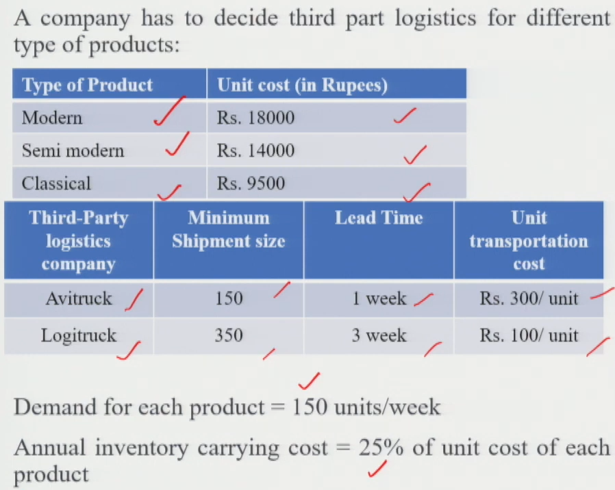
Section titled “Worked Example — 3PL Provider Selection (Total Cost Analysis)”Context: A company is choosing between two logistics providers — Avitruck and Logitruck — for three product types: Modern, Semi-Modern, and Classical.
Input Data Table:
Total Cost Formula:
Sample Calculation — Logitruck + Modern Product:
- Cycle Stock = 0.5 × 350 = 175 units
- Pipeline Inventory = 3 weeks × 150 units/week = 450 units
- Total Inventory = 175 + 450 = 625 units
- Annual Inventory Carrying Cost = 625 × ₹18,000 × 0.25 = ₹28,12,500
- Annual Transport Cost = 150 × 52 × ₹100 = ₹7,80,000
- Total Cost = 28,12,500 + 7,80,000 = ₹35,92,500
Results — All Combinations Analysed:
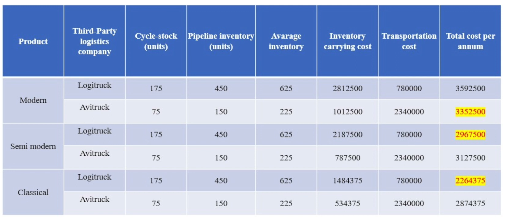
Decision Outcomes:
| Product Type | Recommended Provider | Reason |
|---|---|---|
| Modern | Avitruck | Lower total cost |
| Semi-Modern | Logitruck | Lower total cost |
| Classical | Logitruck | Lower total cost |
Process 6 — Customer Service
Section titled “Process 6 — Customer Service”Role: Customer service drives the entire supply chain — it focuses on providing support to customers throughout their end-to-end experience, from order placement through to post-delivery.
3 Core Customer Expectations:
| Expectation | Description |
|---|---|
| Effective Communication | Real-time order tracking and full visibility into shipment status |
| Responsiveness | Fast responses to queries, complaints, and service issues |
| Quality | Consistently high product and service quality at every touchpoint |
Scope of Digitisation in Customer Service
Section titled “Scope of Digitisation in Customer Service”- Improved inventory management → faster response times → more customers attracted and retained
- Order tracking systems → transparency and visibility for the customer throughout delivery
- Reverse logistics: returns, refunds, and exchanges managed efficiently via digitised systems
Customer Service KPIs — Definitions
Section titled “Customer Service KPIs — Definitions”| KPI | Definition |
|---|---|
| Order Fulfilment Cycle Time | Time elapsed from order placement to final delivery |
| On-Time Delivery (OTD) | Percentage of orders delivered on or before the promised date |
| Fill Rate | Percentage of customer demand fulfilled immediately from stock — no backorders, no delays |
| Return Rate | Percentage of products returned by customers; critical in e-commerce — efficient processing = better experience |
| Supplier On-Time Delivery Rate | Percentage of times the supplier delivers raw materials on time (tracks upstream supplier performance) |
| Compliance with SLAs | Adherence to agreed service level agreements with customers |
Worked Example — Soap Bar Manufacturer
Section titled “Worked Example — Soap Bar Manufacturer”Input data:
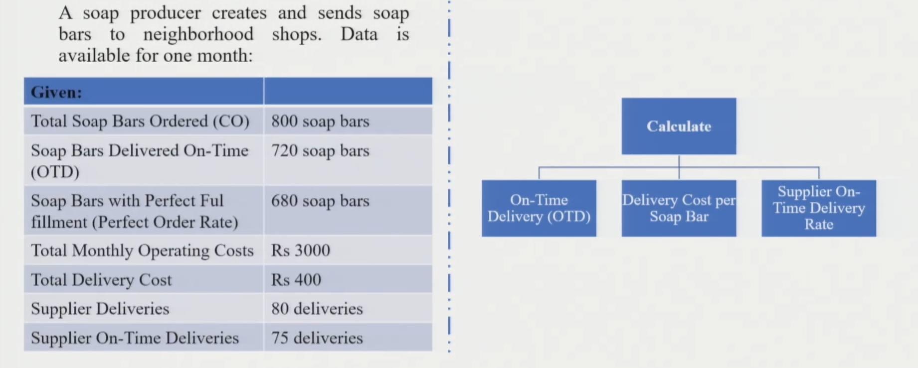
KPI Calculations:
Module 1 — Full Summary Table (All 6 SC Processes)
Section titled “Module 1 — Full Summary Table (All 6 SC Processes)”| Process | Core Goal | Key Techniques | Key KPIs |
|---|---|---|---|
| Planning & Forecasting | Predict demand; plan resources, capacity, and network | Moving Average, Regression, AI/ML | MAPE, MAD, MSE, RMSE, Bias, R² |
| Sourcing & Procurement | Right suppliers at right cost; end-to-end acquisition to payment | Supplier Evaluation, Kraljic Matrix | Supplier Score, Lead Time, PO Cycle Time, PO Accuracy, Compliance |
| Production & Manufacturing | Convert RM to FG efficiently; monitor with data | SPC, ML, Predictive Maintenance | OEE, Cycle Time, Throughput, Utilisation (89.9%), Efficiency (94.8%) |
| Inventory Management | Balance stock availability vs. holding cost | ABC Analysis, Safety Stock, EOQ, Reorder Point | Avg Inventory, Turnover Ratio, Turnover Rate, Stockout Rate, Carrying Cost, Days on Hand |
| Distribution & Logistics | Make product available to the customer efficiently | Route/Fleet/Warehouse Optimisation, 3PL Cost Analysis | Transport Cost/Unit, Order Cycle Time, OTD, Turnover Rate, OTIF |
| Customer Service | Support customers; ensure satisfaction and loyalty | Real-Time Tracking, Reverse Logistics Systems | Fulfilment Cycle Time, OTD, Fill Rate, Return Rate, Supplier OTD, SLA Compliance |