Week 6 | Session 5: Classification Tree in Python — Full Hands-On Code

Course: Supply Chain Digitization — Module 3: Analytics in SCM

Session Agenda

Session Context — Theory to Code

Sessions 3 & 4: Showed the output of the model and explained HOW it is built (Gini, node splitting, stopping criteria)
Session 5: Reproduce the EXACT same output using Python code — closes the loop from theory to implementation
Platform: Google Colab — browser-based Python environment, no local installation needed
Data file: maintenance.csv — 1000 rows, 8 columns (same dataset used in Sessions 3 & 4)
Expected output: Same decision tree structure, same Gini values, same node counts as shown in theory slides

Libraries Used

Library	Import As / From	Purpose in This Model
pandas	`import pandas as pd`	Data manipulation and analysis. Used to read CSV file and create DataFrame.
sklearn (scikit-learn)	`from sklearn import...`	Machine learning library. Provides Decision Tree Classifier, train-test split, confusion matrix, and accuracy score.
matplotlib	`import matplotlib.pyplot as plt`	Plotting library. Used to visualise and print the decision tree diagram.

Complete Code Reference — All Steps Together

Python code implementation

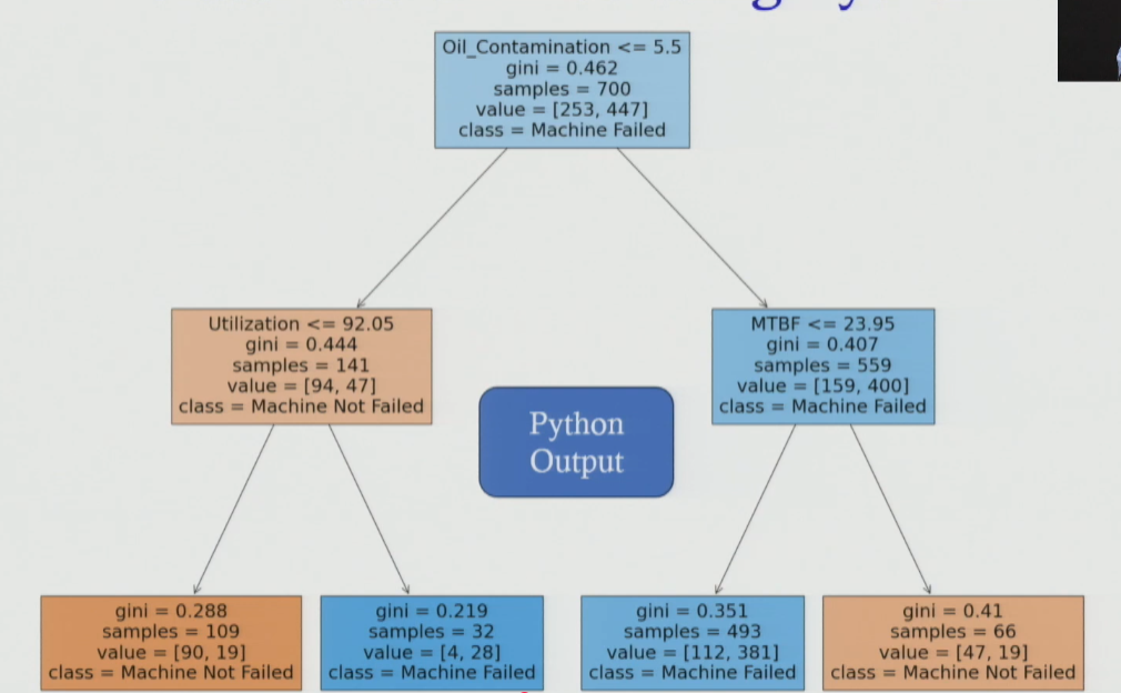
# ── STEP 1: Import Libraries & Data ──────────────────────────
import pandas as pd
import matplotlib.pyplot as plt
from sklearn import tree
from sklearn.tree import DecisionTreeClassifier
from sklearn.model_selection import train_test_split
from sklearn.metrics import confusion_matrix, accuracy_score

df = pd.read_csv("maintenance.csv")

# ── STEP 2: Define Features (X) and Target (Y) ───────────────
X_features = list(df.columns)
X_features.remove("machine_failure")
X = df[X_features]
Y = df["machine_failure"]

# ── STEP 3: Train-Test Split ─────────────────────────────────
X_train, X_test, Y_train, Y_test = train_test_split(
    X, Y, test_size=0.30, random_state=42)

# ── STEP 4: Build Classification Tree ───────────────────────
clf = DecisionTreeClassifier(criterion="gini", max_depth=2)
clf.fit(X_train, Y_train)

# ── STEP 5: Print the Tree ───────────────────────────────────
plt.figure(figsize=(15, 10))
tree.plot_tree(clf,
    feature_names=X_train.columns,
    class_names=["Not Failed", "Failed"],
    filled=True)
plt.show()

# ── STEP 6: Predict & Evaluate ───────────────────────────────
Y_pred = clf.predict(X_test)
cm = confusion_matrix(Y_test, Y_pred)
acc = accuracy_score(Y_test, Y_pred)
print("Confusion Matrix:\n", cm)
print("Accuracy:", acc)

Step-by-Step Breakdown

Step 1 — Import Data

pd.read_csv(): Reads the CSV file and stores it as a DataFrame (df) — a table with labelled rows and columns.
After this step: df has 1000 rows and 8 columns including the target (machine_failure).

Step 2 — Define X (Features) and Y (Target)

X: 7 independent variables (all columns except machine_failure) — used to predict Y.
Y: machine_failure column — what the model must predict (0 = not failed, 1 = failed).

Step 3 — Train-Test Split (70/30)

Why split? If the model is trained and tested on the same data → artificially inflated accuracy (overfitting). Test data must be held out and NEVER used during training.
test_size=0.30: 30% = 300 observations for testing. 70% = 700 for training.

Step 4 — Build the Classification Tree

criterion="gini": Use Gini impurity index to decide which variable and cutoff to split each node.
max_depth=2: Stop splitting after reaching 2 levels from the root. Prevents overfitting. Produces 4 leaf nodes.
clf.fit(X_train, Y_train): Trains the model — the algorithm finds the best splits using 700 training observations.

Step 5 — Visualise the Decision Tree

Output matches Session 3 diagram exactly: Same splits (oil contamination → MTBF / utilisation), same Gini values, same sample counts.
Node 0 (root): 700 samples | Gini = 0.462 | Split: oil_contamination ≤ 5.5

Step 6 — Predict on Test Data and Evaluate Model

6a. Generate Predictions

clf.predict(X_test): Applies the trained model to the 300 test observations — produces predicted Y values.

6b. Confusion Matrix

	Predicted: NOT FAIL (0)	Predicted: FAIL (1)
Actual: NOT FAIL (0)	57 ✓ True Negative	65 ✗ False Positive
Actual: FAIL (1)	16 ✗ False Negative	162 ✓ True Positive

True Negative (57): Model correctly predicted machine did NOT fail — actual also not failed
True Positive (162): Model correctly predicted machine FAILED — actual also failed
False Positive (65): Model predicted FAIL — actual did NOT fail (over-alarm)
False Negative (16): Model predicted NOT FAIL — actual DID fail (missed failure — more dangerous in practice)

6c. Accuracy Score

Accuracy = 73%: 73 out of every 100 test instances are predicted correctly. (57 + 162) / 300 = 0.73.
Compare to baseline: If model always predicted “FAIL” (majority class, 64%) → 64% accuracy. Model achieves 73% → meaningful improvement.

How to Run in Google Colab

Open browser → go to colab.research.google.com → sign in with Google account
New notebook → upload maintenance.csv using the file upload icon (left sidebar)
Copy and paste the complete code above into a code cell
Run cells sequentially (Shift + Enter or click the ▶ button)
Decision tree diagram rendered in the output area. Confusion matrix and accuracy printed below.

Session Summary

Session 3: Case study setup + decision tree OUTPUT — 4 leaf nodes, business rules, 2 worked predictions
Session 4: HOW the tree is built — Gini index, entropy, node splitting logic, stopping criteria, overfitting
Session 5 (this session): Python implementation — 6-step code, exact same output verified, confusion matrix, 73% test accuracy
Next module: AI/ML for demand forecasting — further predictive analytics applications in SCM