Week 2 | Session 4: Analytical Product Segmentation & Kraljic Matrix
Course: Supply Chain Digitization
Session Context
Section titled “Session Context”Part 1 — Analytical Product Segmentation: Demand Variability & Weekly Sales
Section titled “Part 1 — Analytical Product Segmentation: Demand Variability & Weekly Sales”Case Setup
Section titled “Case Setup”Company: Electronic gadgets manufacturer with a large variety of SKUs. Products: Smartphones, tablets, smart watches, and other gadgets. Operations: 2 cities — City A and City B; 2 channels — Online and Retail. Data available: Weekly sales for 20 SKUs over 8 weeks for both cities. Annual revenue: USD 1 billion.
Segmentation variables used:
| Variable | What It Measures |
|---|---|
| Average Weekly Sales | Volume indicator — how much of a SKU is sold per week on average |
| Demand Variability / Order Variability | Stability indicator — how much demand fluctuates from week to week |
Measuring Demand Variability — Coefficient of Variation (CoV)
Section titled “Measuring Demand Variability — Coefficient of Variation (CoV)”Formulas:
Steps to Calculate & Segment (Excel-Based Workflow)
Section titled “Steps to Calculate & Segment (Excel-Based Workflow)”- Collect data — gather 8-week weekly demand data for all 20 SKUs for City A and City B separately
- Calculate SKU-wise average demand — use the
AVERAGEIFSconditional formula for each city - Calculate SKU-wise standard deviation — use the
STDEVIFSconditional formula for each city - Compute CoV — divide σ by μ for each SKU per city:
CoV = σ / μ - Plot a scatter — X-axis: CoV (demand variability); Y-axis: Average weekly sales — one scatter per city
- Combine City A + City B demand — compute the joint average demand, joint σ, and joint CoV for each SKU
- Plot the combined (joint) scatter — this represents the Distribution Centre view serving both cities
- Build the 4-Quadrant Matrix — assign an SC strategy to each product group based on quadrant position
Raw Weekly Sales Data Table
Section titled “Raw Weekly Sales Data Table”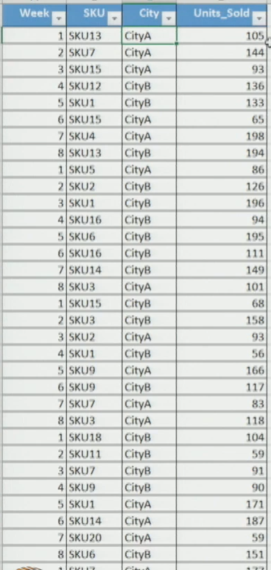
CoV Calculations — City A
Section titled “CoV Calculations — City A”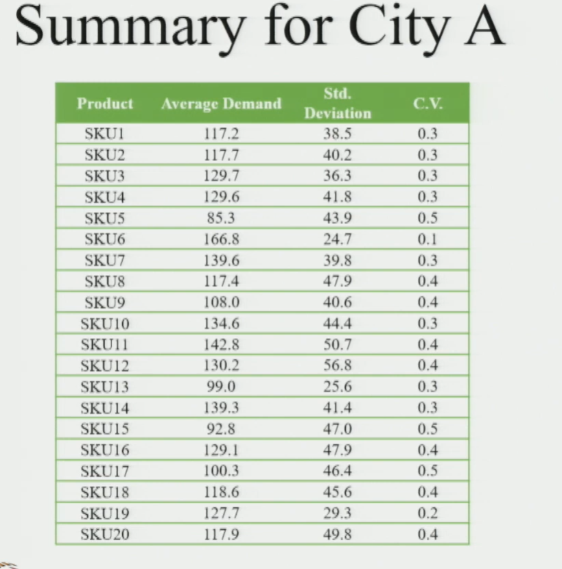
CoV Calculations — City B
Section titled “CoV Calculations — City B”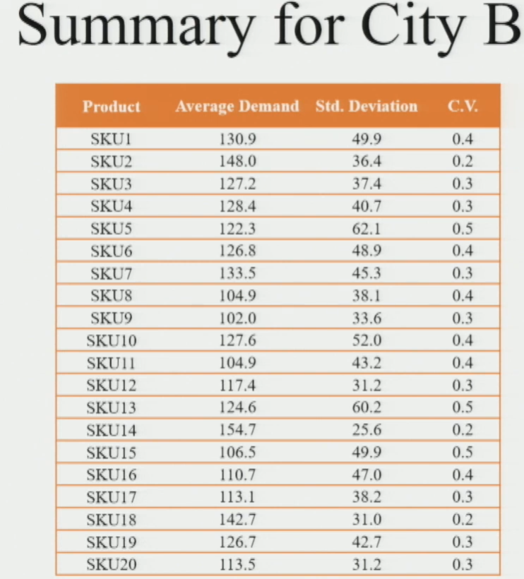
Joint (Combined) CoV — Distribution Centre View
Section titled “Joint (Combined) CoV — Distribution Centre View”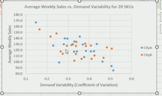
Scatter Plot — City A & City B Combined
Section titled “Scatter Plot — City A & City B Combined”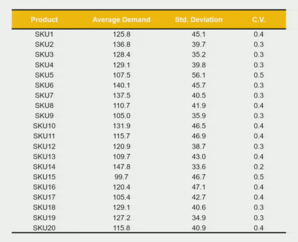
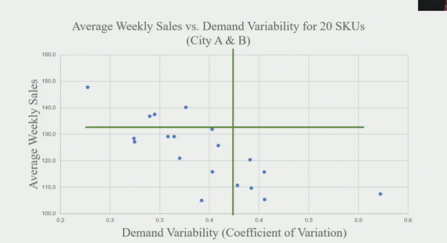
Scatter Plot — Distribution Centre (Joint) View
Section titled “Scatter Plot — Distribution Centre (Joint) View”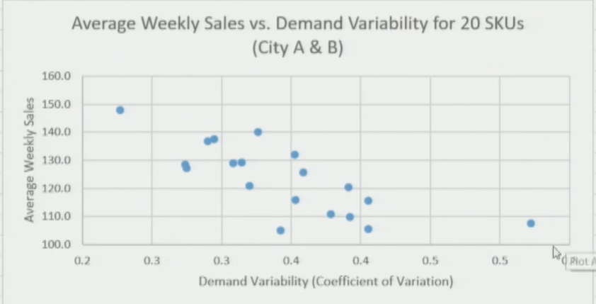
4-Quadrant Strategy Matrix
Section titled “4-Quadrant Strategy Matrix”The scatter plots are divided into four quadrants based on threshold values for CoV and average weekly sales. Each quadrant maps to a distinct SC strategy.
Quadrant 1 — Low CoV + High Sales (Top-Left)
Section titled “Quadrant 1 — Low CoV + High Sales (Top-Left)”| Attribute | Detail |
|---|---|
| Product type | Essential / High-volume products |
| Characteristics | Always in demand, stable, predictable |
| Examples | Standard commodity goods, staple consumer products |
| SC type | Efficient Supply Chain |
| Strategy | PUSH — forecast-driven, mass production |
Quadrant 2 — High CoV + Low Sales (Bottom-Right)
Section titled “Quadrant 2 — High CoV + Low Sales (Bottom-Right)”| Attribute | Detail |
|---|---|
| Product type | Customised / Niche products |
| Characteristics | Low demand volume + high unpredictability |
| Examples | Special-edition collectibles, highly customised products |
| SC type | Responsive Supply Chain |
| Strategy | PULL — demand-driven, high customisation |
Quadrant 3 — High CoV + High Sales (Top-Right)
Section titled “Quadrant 3 — High CoV + High Sales (Top-Right)”| Attribute | Detail |
|---|---|
| Product type | Consumer electronics / High-tech products |
| Characteristics | High volume AND high variability — the most complex quadrant to manage |
| Examples | Consumer electronics, tech gadgets with rapid model changes |
| Strategy | Hybrid Push-Pull — apply push-pull boundary framework from Session 3; boundary position depends on level of customisation required |
Quadrant 4 — Low CoV + Low Sales (Bottom-Left)
Section titled “Quadrant 4 — Low CoV + Low Sales (Bottom-Left)”| Attribute | Detail |
|---|---|
| Product type | Basic / Slow-moving products |
| Characteristics | Low sales + stable demand — neither high priority nor high risk |
| Examples | Non-seasonal apparel basics, basic electronic components |
| Strategy | Hybrid Push-Pull — specific combination determined by individual product requirements |
Part 2 — Kraljic Matrix: Procurement & Sourcing Segmentation
Section titled “Part 2 — Kraljic Matrix: Procurement & Sourcing Segmentation”Two Axes of the Kraljic Matrix
Section titled “Two Axes of the Kraljic Matrix”| Axis | What It Measures | Key Factors |
|---|---|---|
| X-axis — Supply Risk | How difficult or risky it is to procure the component | Availability of the component; number of suppliers; competitive demand; make-or-buy feasibility; other supply-side risk factors |
| Y-axis — Profit Impact | How significantly the component affects business profitability | Volume required; percentage of total purchase cost; direct or indirect impact on business growth |
4 Quadrants of the Kraljic Matrix
Section titled “4 Quadrants of the Kraljic Matrix”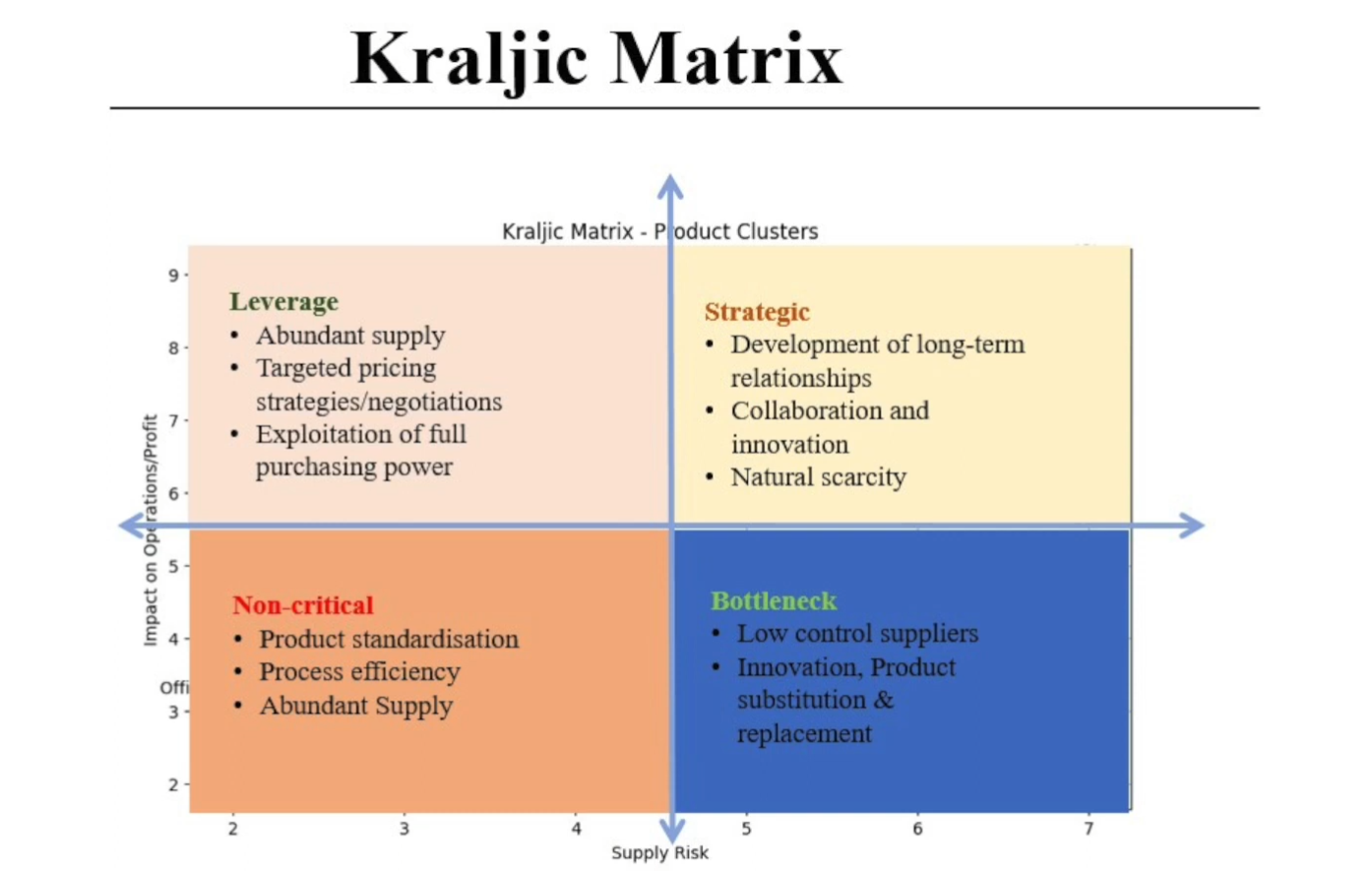
1. Non-Critical Items — Low Supply Risk + Low Profit Impact
Section titled “1. Non-Critical Items — Low Supply Risk + Low Profit Impact”| Attribute | Detail |
|---|---|
| Characteristics | Highly standardised; abundant supply — many suppliers available; easy to manage |
| Strategy | Streamline procurement — reduce administrative effort, automate ordering where possible |
2. Leverage Items — Low Supply Risk + High Profit Impact
Section titled “2. Leverage Items — Low Supply Risk + High Profit Impact”| Attribute | Detail |
|---|---|
| Characteristics | Abundant supply available but high impact on profit; company holds strong purchasing power |
| Strategy | Exploit full purchasing power — competitive bidding, aggressive price negotiation, good pricing strategy |
3. Strategic Items — High Supply Risk + High Profit Impact
Section titled “3. Strategic Items — High Supply Risk + High Profit Impact”| Attribute | Detail |
|---|---|
| Characteristics | Most critical category — high risk AND high profit impact; affects the business on a long-term basis; cannot switch suppliers easily |
| Strategy | Long-term supplier relationships + deep collaboration — partnership approach, joint development, strategic alliances; focus on supply continuity |
4. Bottleneck Items — High Supply Risk + Low Profit Impact
Section titled “4. Bottleneck Items — High Supply Risk + Low Profit Impact”| Attribute | Detail |
|---|---|
| Characteristics | High supply risk but minimal direct profit impact; very low control over suppliers; unavailability can still disrupt operations even when profit impact is low |
| Strategy | Ensure availability through safety stock and alternate sourcing; monitor closely |
Kraljic Matrix — Quick Reference
Section titled “Kraljic Matrix — Quick Reference”| Quadrant | Supply Risk | Profit Impact | Procurement Strategy |
|---|---|---|---|
| Non-Critical | Low | Low | Streamline and automate procurement |
| Leverage | Low | High | Negotiate hard; competitive bidding |
| Strategic | High | High | Long-term partnerships; deep collaboration |
| Bottleneck | High | Low | Secure supply; hold safety stock; monitor closely |
Session Summary — Two Analytical Tools
Section titled “Session Summary — Two Analytical Tools”| Tool | Axes | Output | Strategy Assigned |
|---|---|---|---|
| Demand Variability vs. Weekly Sales Quadrant | X: CoV (variability), Y: Avg weekly sales | 4-quadrant product classification | Q1 = Push | Q2 = Pull | Q3 & Q4 = Hybrid Push-Pull |
| Kraljic Matrix | X: Supply risk, Y: Profit impact | 4-quadrant component classification | Non-Critical = Streamline | Leverage = Negotiate | Strategic = Partner | Bottleneck = Secure |