Week 11 | Session 3: GFA Hands-On — Excel Solver Formulas & AnyLogistix (Multi-SKU)

Course: Supply Chain Digitization — Module 4: Digital Infrastructure

Session Agenda

1. Case Reminder

Parameter	Value
4 markets	Pune (M1), Mumbai (M2), Ahmedabad (M3), Surat (M4)
Known	Annual demand + latitude/longitude per market
Unknown	xDC (latitude), yDC (longitude) of the new DC
Objective	Minimize Z = Σ (Demand_i × Distance_i × $1/km/unit)
Initial DC	lat = 20, long = 72 → Z = 12,44,89,119 (not optimal)

2. Excel — Formula Build-Up (Spherical Distance)

Excel Formula Setup — GFA Spherical Distance

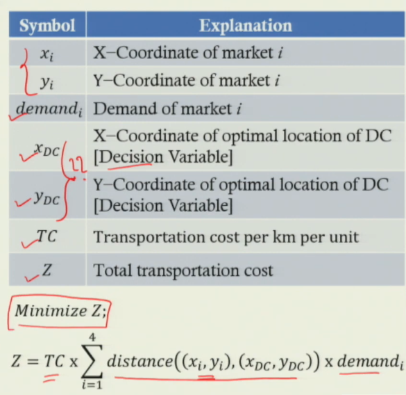
The distance formula requires 5 intermediate calculations before arriving at km distance.

Key cell references: B7 = xDC (lat of DC), B8 = yDC (long of DC), D2 = xᵢ (lat of market i), E2 = yᵢ (long of market i).

Step	Cell / Variable	Excel Formula	Explanation
1	`d_long`	`=RADIANS(B8 − E2)`	Difference in longitude, converted to radians
2	`d_lat`	`=RADIANS(B7 − D2)`	Difference in latitude, converted to radians
3	`A`	`=SIN(d_lat/2)^2 + COS(RADIANS(D2)) * COS(RADIANS(B7)) * SIN(d_long/2)^2`	Haversine intermediate term
4	`C`	`=2 * ATAN2(SQRT(1−A), SQRT(A))`	Central angle in radians (two-argument arctangent)
5	`Distance`	`=6371 * C`	Distance in km = Earth’s radius (6371 km) × central angle
6	`Total Cost`	`=SUMPRODUCT(distances_range, demands_range, cost_range)`	One formula gives total cost across all 4 markets

Step-by-Step Formula Chain (for Market 1 = Pune)

Step 1 — d_long   = RADIANS(B8 − E2)
Step 2 — d_lat    = RADIANS(B7 − D2)
Step 3 — A        = SIN(d_lat/2)^2 + COS(RADIANS(D2)) * COS(RADIANS(B7)) * SIN(d_long/2)^2
Step 4 — C        = 2 * ATAN2(SQRT(1−A), SQRT(A))
Step 5 — Distance = 6371 * C    [km, accounts for earth curvature]
Step 6 — Total Cost = SUMPRODUCT(distances, demands, costs)

Apply the same formula for all 4 markets (rows 2–5) by changing D2→D3, E2→E3, etc. B7 and B8 remain fixed throughout — they are the decision variables.

3. Excel Solver — Settings & Output

Excel Solver Configuration

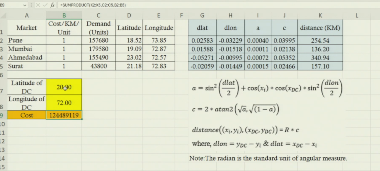
Solver Field	Value / Setting
Set Objective	Cell B9 (Total Cost)
To	Min (Minimize)
By Changing Variable Cells	B7:B8 (Latitude and Longitude of DC)
Subject to Constraints	None — DC can be placed anywhere
Solving Method	GRG Non-linear — spherical formula is non-linear
Optimal Output	B7 = 19.09 (lat), B8 = 72.87 (long) → Mumbai
Minimized Cost	₹9,73,92,135 (vs ₹12,44,89,119 at initial 20, 72)

Tip: Install Solver via Data tab. If not visible: File → Options → Add-ins → Manage Excel Add-ins → check Solver Add-in → OK.

After solving: Mumbai distance = 0 (DC placed exactly at Mumbai coordinates) — confirms solution.

4. Advanced Scenario — Multiple SKUs & Daily Demand

Why Complexity Increases

Scenario	Demand entries
Session 2 (basic)	1 product × 4 markets = 4 entries (annual)
Session 3 (advanced)	4 SKUs × 4 markets = 16 entries (daily demand)
Real companies	20–100 SKUs × thousands of markets → Excel cannot handle

Excel limitation: cannot solve LP/NLP models with more than ~200 decision variables efficiently. Solution: use AnyLogistix software.

Multi-SKU Demand Data (Advanced Case — Daily Demand)

Market	SKU1 (units/day)	SKU2 (units/day)	SKU3 (units/day)	SKU4 (units/day)	Coordinates
Pune	130	90	95	—	18.52, 73.85
Mumbai	—	—	—	—	19.09, 72.87
Ahmedabad	—	—	—	—	23.02, 72.57
Surat	—	—	—	—	21.18, 72.83

(Full SKU demand per market entered in AnyLogistix)

5. AnyLogistix — GFA Step-by-Step (Hands-On)

AnyLogistix Multi-SKU Input

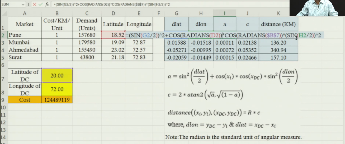
Download & Install: Go to anylogic.com → Academic tab → ALX Educational Toolkit → download AnyLogistix Personal Learning Edition (PLE) — free for students.
Open GFA Module: Launch AnyLogistix → Select ‘Green Field Analysis’ module (vs Network Optimization or Simulation).
Enter Customer Data: Add 4 customers: Pune, Mumbai, Ahmedabad, Surat. Enter lat/long manually OR type city name → auto-fill coordinates from database.
Enter Demand Data: For each customer, enter daily demand per SKU. 4 SKUs × 4 markets = 16 demand entries (e.g., Pune SKU1 = 130 units/day).
Enter Product Data: Define products: SKU1, SKU2, SKU3, SKU4 with unit type. Can add more SKUs as needed.
Run GFA Experiment: Click Run → optimizer automatically runs the spherical-distance weighted demand model → output in seconds.
Read Output: Optimal DC: lat 19.096, long 72.877 (Mumbai). Map shows DC location with connections to all 4 customers.
Explore Flows: View flow table: DC → Ahmedabad, SKU1: 43,800 units, distance 437.988 km, flow cost shown. All 16 SKU-market flows visible.

Auto Lat/Long Feature

If city name is entered correctly → AnyLogistix auto-fills coordinates from its internal database. Eliminates manual lat/long lookup — critical advantage at large scale.

6. Excel vs AnyLogistix — Output Comparison

AnyLogistix GFA Map Output

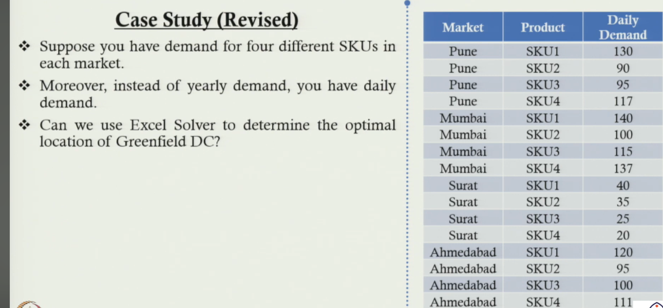
Output / Feature	Excel Solver	AnyLogistix
Optimal Latitude	19.09	19.096
Optimal Longitude	72.87	72.877
Location	Mumbai	Mumbai
Map visualization	No (cell values only)	Yes — on geographic map
Flow breakdown	No	Yes — per SKU per route
Multi-SKU support	Limited	Yes — 4+ SKUs
Scale feasible	~4 markets only	Thousands of markets

Both tools give identical optimal location (lat 19.09, long 72.87) — confirms model correctness. AnyLogistix adds: map visualization, flow breakdown per SKU per route, scalability to thousands of markets.

Session Summary

Excel formula chain: d_long → d_lat → A → C → Distance (= 6371 × C) → SUMPRODUCT for total cost.
Key cells: B7 = xDC, B8 = yDC (decision variables). B9 = total cost (objective). D2:E5 = market coordinates.
Solver: Minimize B9, changing B7:B8, GRG Non-linear, no constraints → optimal: 19.09, 72.87 (Mumbai).
Advanced case: 4 SKUs × 4 markets = 16 demands, daily demand — Excel too limited → AnyLogistix needed.
AnyLogistix: Enter city names → auto lat/long → enter daily SKU demand → Run GFA → map + flow output instantly.
Both outputs agree: DC optimal location = lat 19.096, long 72.877 = Mumbai.