Week 2 | Session 5: Inventory Segmentation — Methods, Advanced Approaches & AHP Case
Course: Supply Chain Digitization
Recap & Session Context
Section titled “Recap & Session Context”What is Inventory Segmentation?
Section titled “What is Inventory Segmentation?”Key benefits:
| Benefit | Description |
|---|---|
| Cost optimisation | Allocate SC resources precisely where they generate the most value |
| Improved service levels | Set and maintain the right service level per SKU category |
| Right storage system | Assign appropriate storage infrastructure per inventory type |
| Better picking strategy | Design warehouse and DC picking processes based on movement frequency and item characteristics |
| Operational performance | Overall improvement across fulfilment, replenishment, and inventory accuracy |
Popular Inventory Segmentation Methods — 4 Traditional Approaches
Section titled “Popular Inventory Segmentation Methods — 4 Traditional Approaches”1. ABC Analysis — Revenue-Based
Section titled “1. ABC Analysis — Revenue-Based”Classification based on the revenue contribution of each inventory item — the Pareto principle applied to inventory.
| Segment | Share of Products | Share of Revenue | Management Priority |
|---|---|---|---|
| A | ~20% | ~80% | Highest — tightly monitored, frequent review |
| B | ~30% | ~15% | Moderate — regular review |
| C | ~50% | ~5% | Lowest — simplified, automated management |
2. FSN Analysis — Movement-Based
Section titled “2. FSN Analysis — Movement-Based”Classification based on the consumption rate and speed of movement through the warehouse.
| Segment | Share of Items | Movement Behaviour | Avg Cumulative Stay |
|---|---|---|---|
| F — Fast Moving | ~10% | Very short stay in warehouse; consumed rapidly | Less than 10% of average cumulative stay |
| S — Slow Moving | ~30% | Moderate movement; stays longer in warehouse | ~20% of average cumulative stay |
| N — Non-Moving | ~50% | Stagnant inventory — no consumption for extended period; inventory turnover ratio < 1 | High cumulative stay |
3. VED Analysis — Criticality-Based
Section titled “3. VED Analysis — Criticality-Based”Classification based on the criticality of each item to business operations — not its value or movement speed.
| Segment | Meaning | Description |
|---|---|---|
| V — Vital | Cannot operate without it | Absolutely crucial — business halts if unavailable |
| E — Essential | Very important | High priority after Vital; significant disruption if unavailable |
| D — Desirable | Not strictly necessary | Operations can continue without it, but quality or efficiency suffers |
4. XYZ Analysis — Demand Variability-Based
Section titled “4. XYZ Analysis — Demand Variability-Based”Classification based on the predictability of demand over time — complementary to ABC analysis.
| Segment | Demand Behaviour | Management Approach |
|---|---|---|
| X | Little or no variation — highly predictable | Lean inventory; tight replenishment cycles |
| Y | Unsteady demand — but can be predicted to a certain extent | Moderate safety stock; regular review |
| Z | Very high variation — no discernible trend or causal factors | High safety stock; frequent monitoring; hardest to manage |
Quick Reference — 4 Traditional Methods
Section titled “Quick Reference — 4 Traditional Methods”| Method | Classification Criterion | Segments |
|---|---|---|
| ABC | Revenue contribution | A (high) / B (medium) / C (low) |
| FSN | Speed of movement / consumption rate | F (fast) / S (slow) / N (non-moving) |
| VED | Criticality to operations | V (vital) / E (essential) / D (desirable) |
| XYZ | Demand predictability / variability | X (stable) / Y (variable) / Z (unpredictable) |
Advanced Inventory Segmentation Approaches
Section titled “Advanced Inventory Segmentation Approaches”1. Mathematical Programming
Section titled “1. Mathematical Programming”- Linear Programming (LP) or Non-Linear Programming (NLP)
- Formulates the segmentation problem as a mathematical optimisation model incorporating multiple criteria simultaneously
2. Metaheuristics
Section titled “2. Metaheuristics”Used when the problem is too complex for exact mathematical programming:
| Algorithm | Type |
|---|---|
| Genetic Algorithm (GA) | Evolutionary optimisation |
| Particle Swarm Optimisation (PSO) | Swarm intelligence |
| Simulated Annealing | Probabilistic local search |
3. AI / Machine Learning
Section titled “3. AI / Machine Learning”Heavily data-driven — well suited to today’s data-rich SC environment:
| Algorithm | Type |
|---|---|
| Artificial Neural Networks (ANN) | Deep learning |
| Support Vector Machines (SVM) | Supervised classification |
| Back Propagation Networks | Neural network training |
| K-Nearest Neighbor (KNN) | Instance-based learning |
| Regression models | Predictive modelling |
4. Multi-Criteria Decision Making (MCDM)
Section titled “4. Multi-Criteria Decision Making (MCDM)”Incorporates expert opinion to weigh multiple factors:
| Method | Description |
|---|---|
| AHP — Analytical Hierarchy Process | Pairwise comparison of criteria to derive priority weights |
| Fuzzy AHP | AHP with fuzzy logic to handle uncertainty in expert judgement |
| ANP — Analytical Network Process | Extension of AHP allowing interdependencies between criteria |
5. Hybrid Approaches
Section titled “5. Hybrid Approaches”Combinations of the above — e.g., AHP + ML, GA + LP — used when no single method is adequate alone.
AHP — Analytical Hierarchy Process
Section titled “AHP — Analytical Hierarchy Process”Core Idea
Section titled “Core Idea”AHP organises a complex, multi-factor decision into a hierarchical structure, performs pairwise comparisons of all factors to determine their relative importance, and outputs quantitative, consistent priority weights for each factor. Inputs can come from a single expert or aggregated from multiple experts.
AHP Hierarchy Structure
Section titled “AHP Hierarchy Structure”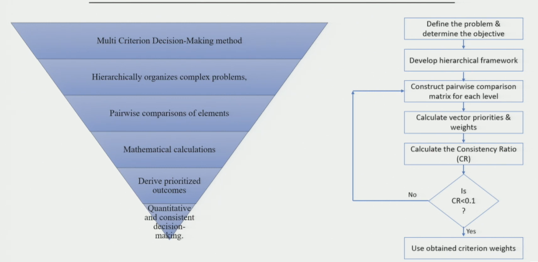
Saaty Scale (1–9)
Section titled “Saaty Scale (1–9)”AHP Steps
Section titled “AHP Steps”- Define the problem — state the objective clearly
- Develop the hierarchical framework — list all criteria and map their relationships
- Construct the Pairwise Comparison Matrix for each level using the Saaty scale (1–9)
- Normalise the matrix — calculate criterion weights (the priority vector)
- Calculate the Consistency Ratio (CR) using:
CR = CI / RIwhere CI = Consistency Index and RI = Random Index (standard table value based on matrix size) - Check CR: If CR < 0.1 → consistent, proceed. If CR ≥ 0.1 → inconsistent, return to Step 3 and redo the pairwise comparison
Case Study — AHP-Based Inventory Segmentation: XYZ E-tailer
Section titled “Case Study — AHP-Based Inventory Segmentation: XYZ E-tailer”Case Setup
Section titled “Case Setup”| Parameter | Detail |
|---|---|
| Company | XYZ E-tail — an e-commerce retailer |
| Constraint | Fixed warehouse space under a 3-year contract |
| Listing policy | A product is listed as ‘available’ only if it is physically present in the warehouse |
| Challenge | Management wants to expand the product portfolio but warehouse space is limited |
| Previous policy | 95% service level maintained uniformly for all SKUs |
| New plan | Classify 25 SKUs into 3 groups with differentiated service levels |
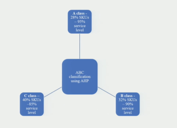
| Tool | AHP — to classify 25 SKUs into Class A / B / C |
Target service levels under the new classification:
| Class | Service Level |
|---|---|
| A | 95% |
| B | 90% |
| C | 85% |
SKU Data — 25 SKUs Across 6 Criteria
Section titled “SKU Data — 25 SKUs Across 6 Criteria”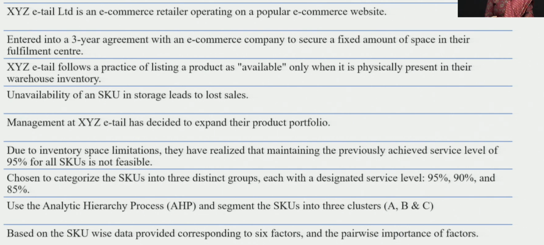
6 Evaluation Criteria
Section titled “6 Evaluation Criteria”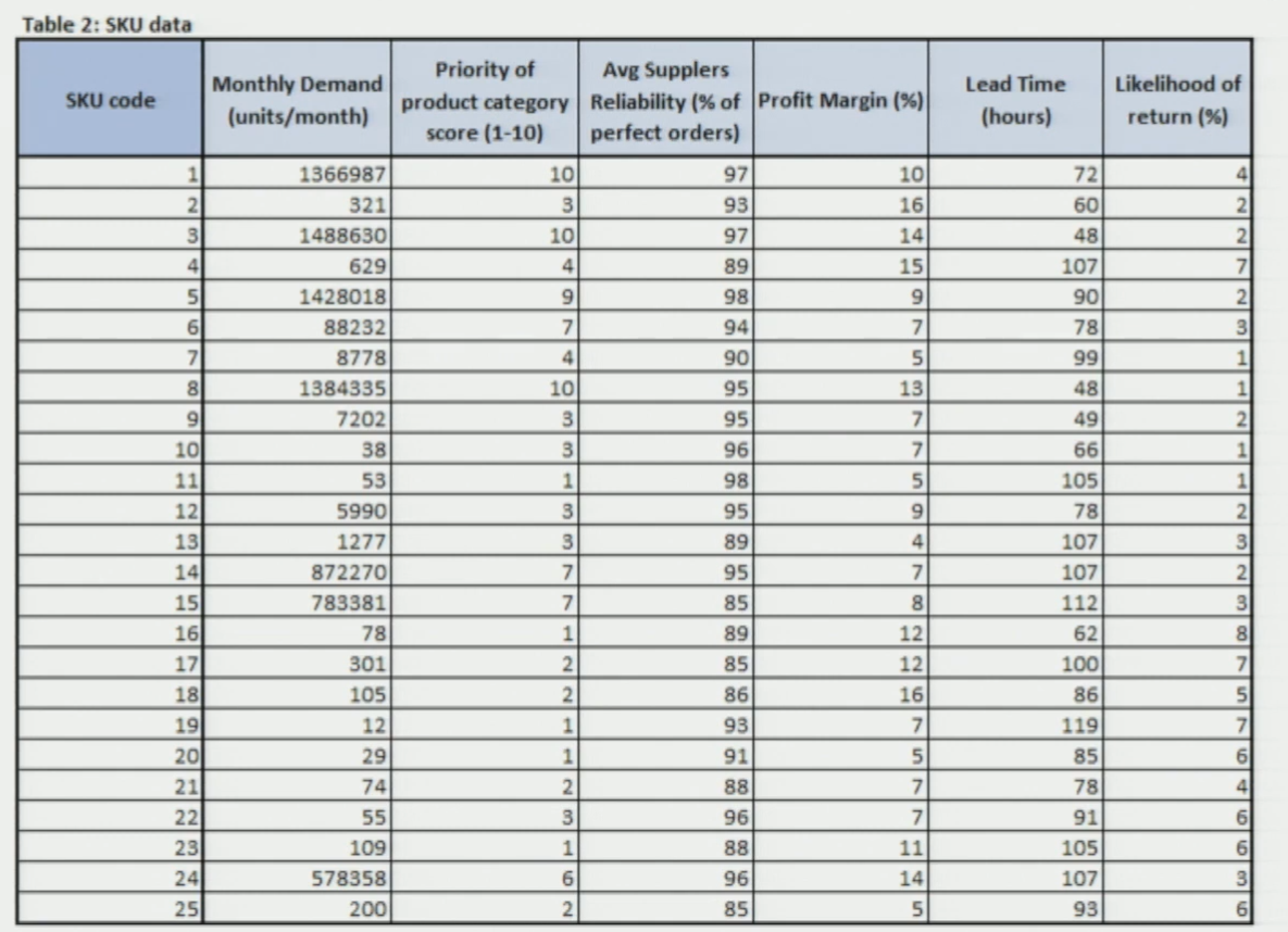
The six criteria used, with their direction of preference:
| # | Criterion | Unit | Direction |
|---|---|---|---|
| 1 | Monthly Demand | Units/month | Higher = Better |
| 2 | Priority of Product Category | Score 1–10 | Higher = Better |
| 3 | Supplier Reliability | % perfect orders | Higher = Better |
| 4 | Profit Margin | % | Higher = Better |
| 5 | Lead Time | Hours | Lower = Better |
| 6 | Likelihood of Return | % | Lower = Better |
Step 1 — Pairwise Comparison Matrix
Section titled “Step 1 — Pairwise Comparison Matrix”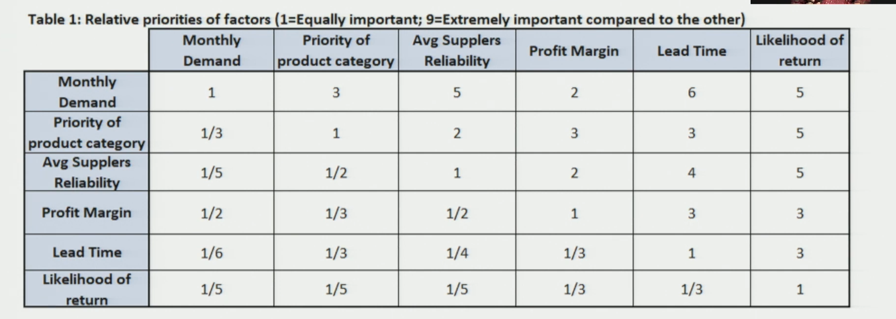
Example reading: Monthly Demand vs. Priority of Product Category → Monthly Demand rated 3× more important (Saaty scale = 3).
Step 2 — Normalised Matrix & Criterion Weights
Section titled “Step 2 — Normalised Matrix & Criterion Weights”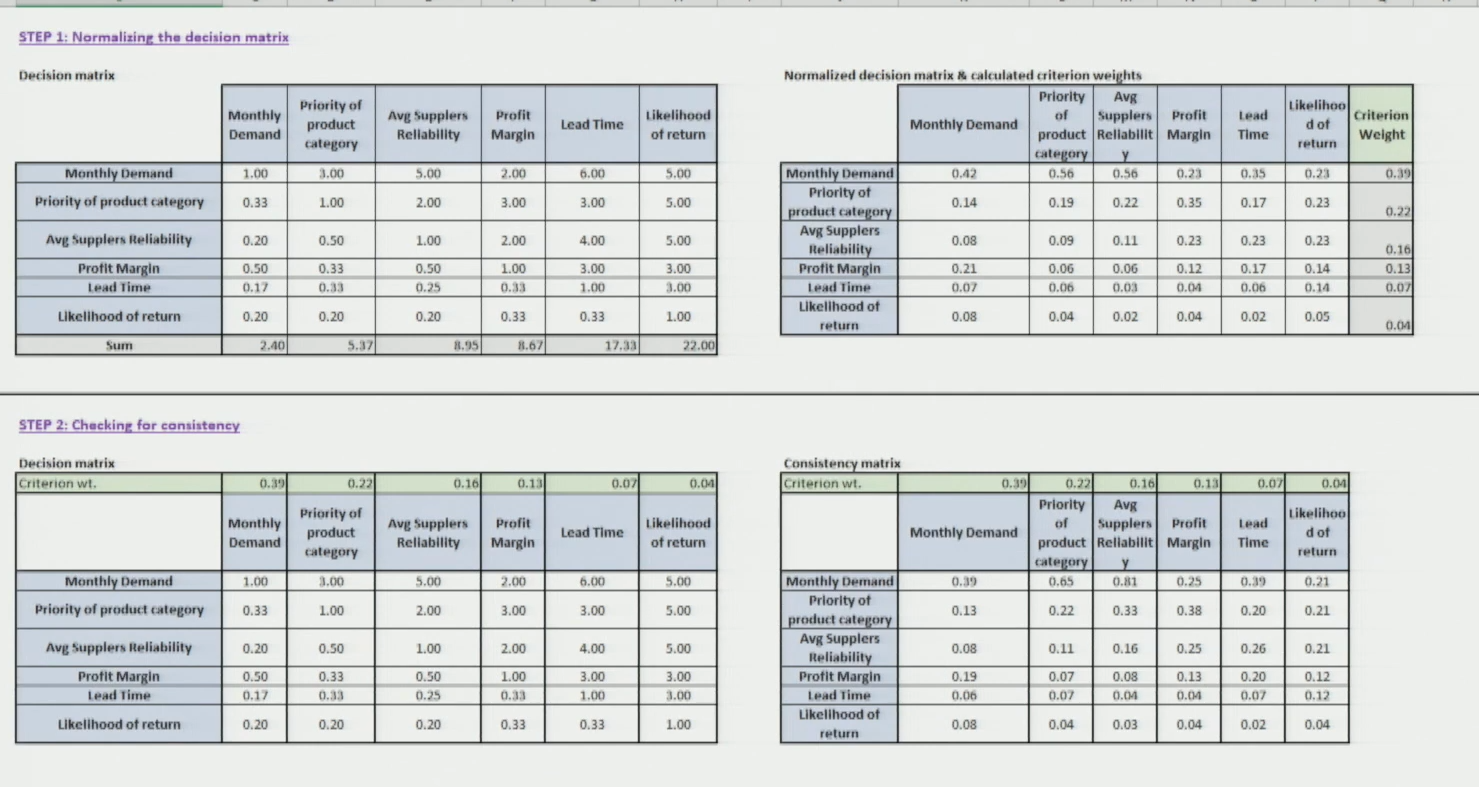
Step 3 — Consistency Check
Section titled “Step 3 — Consistency Check”Criterion Weights Output
Section titled “Criterion Weights Output”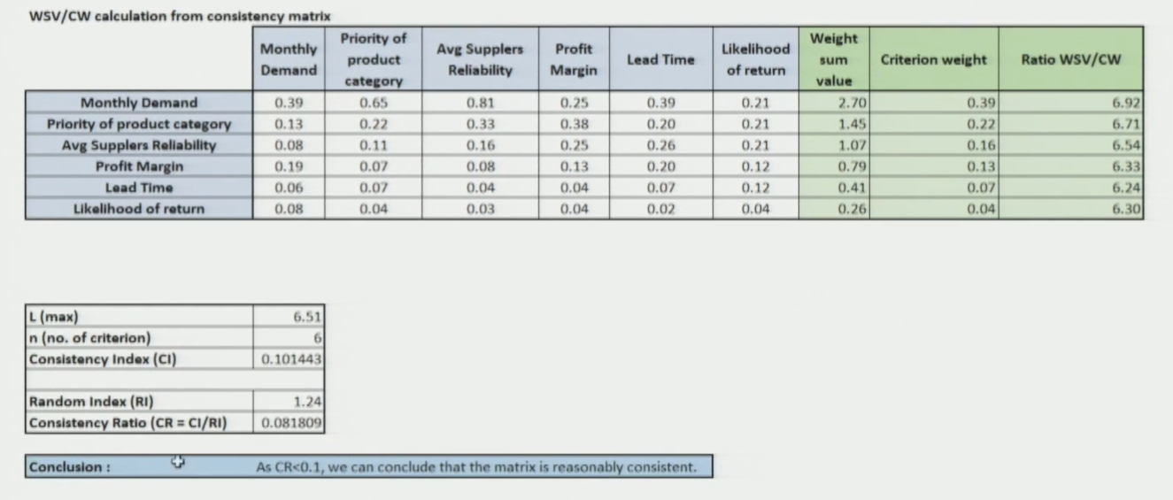
Normalisation of SKU Data
Section titled “Normalisation of SKU Data”Problem: All six criteria are in different units — they cannot be directly compared or multiplied.
Solution: Normalise all criteria to a 0–1 scale before scoring.
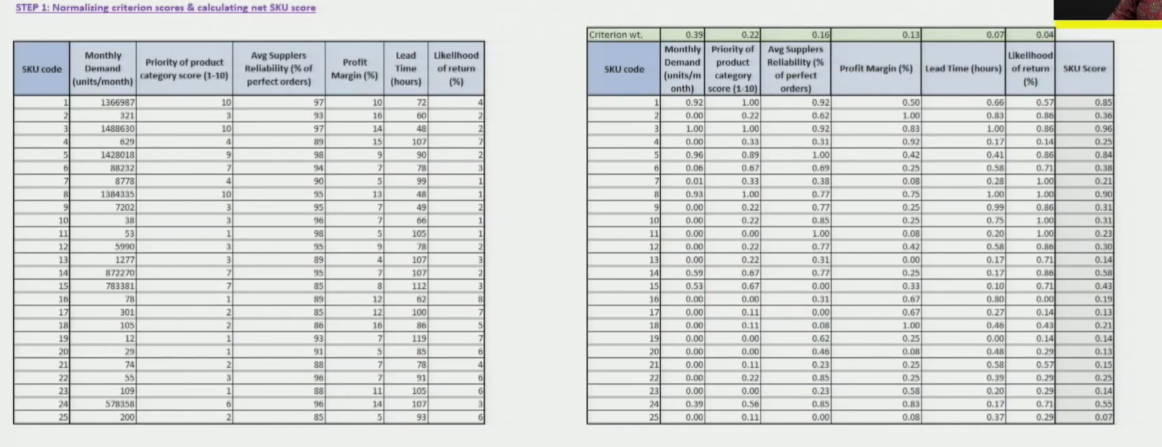
Calculating the SKU Score
Section titled “Calculating the SKU Score”ABC Classification from SKU Scores
Section titled “ABC Classification from SKU Scores”- Sort all 25 SKUs by combined SKU Score in descending order (highest → most important)
- Calculate cumulative score and the cumulative % of total score for each SKU
- Apply cut-offs to assign classes:
- Class A → top SKUs up to ~60% of cumulative score → 7 out of 25 items → 95% service level
- Class B → next ~25% of cumulative score → 8 out of 25 items → 90% service level
- Class C → remaining ~15% → 10 out of 25 items → 85% service level
Final Classification Results
Section titled “Final Classification Results”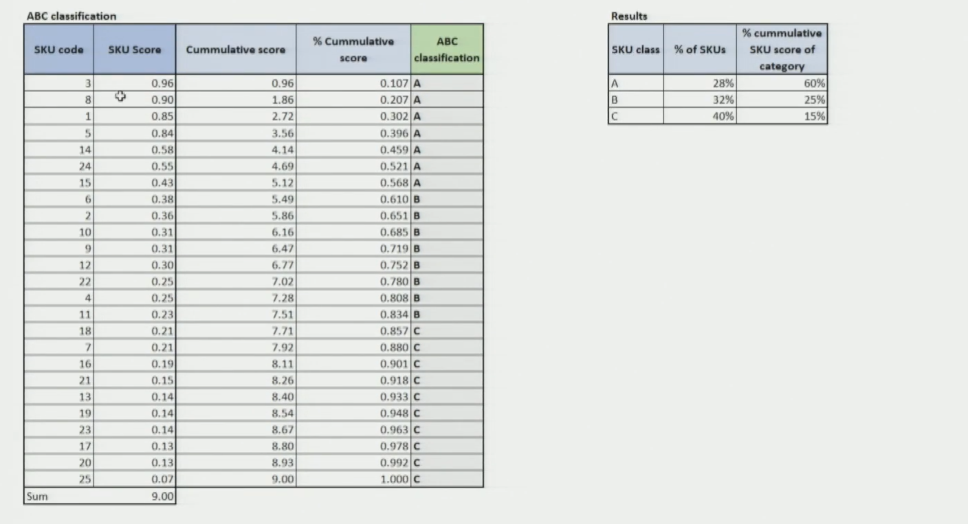
Module 2 Summary — Supply Chain Segmentation (All 5 Sessions)
Section titled “Module 2 Summary — Supply Chain Segmentation (All 5 Sessions)”| Session | Topic Covered |
|---|---|
| Session 1 | SC challenges — building the case for why segmentation is needed |
| Session 2 | 8 reasons for segmentation + 7 types of segmentation |
| Session 3 | Functional vs. Innovative products → Efficient vs. Responsive SC → Push / Pull / Hybrid → Push-Pull Boundary |
| Session 4 | Analytical product segmentation (CoV quadrant) + Kraljic Matrix |
| Session 5 | Inventory segmentation — ABC / FSN / VED / XYZ + Advanced methods + AHP multi-criteria classification case |