Week 9 | Session 5: DEA — Linearization, Excel Solver & Interpretation of Results

Course: Supply Chain Digitization — Module 3: Analytics in SCM

Session Agenda

1. Recap — Session 4

DEA model formulated: Maximize weighted output ÷ weighted input for each facility, subject to all facilities’ efficiency ≤ 1.
Problem: The model is non-linear — decision variables appear in both numerator and denominator.
This session: Linearize the model, solve in Excel Solver, and interpret results.

2. Converting Non-linear DEA to Linear Programming

Linearization of DEA Model

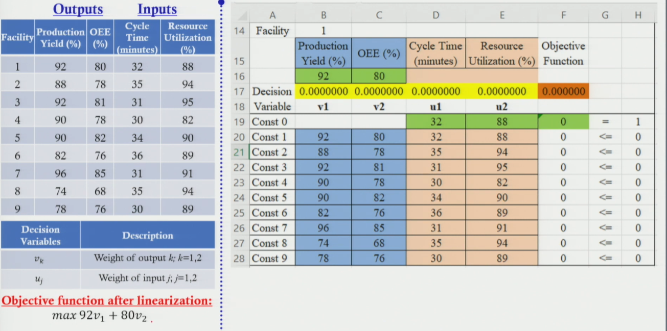
Why non-linear? Both numerator (V1·Y1 + V2·Y2) and denominator (U1·X1 + U2·X2) contain decision variables → Y/X type = non-linear. Strategy: Apply two separate transformations.

Transformation	Why it works
1. Constraint (Non-linear to Linear): `(V·Y) / (U·X) ≤ 1` → `V·Y − U·X ≤ 0`	Cross-multiply denominator to right side. Denominator is positive, so inequality direction stays.
2. Objective (Non-linear to Linear): Maximize `(V·Y) / (U·X)` Add constraint: `U·X = 1` → Linear objective: Maximize `V·Y`	Fix denominator = 1 via an extra equality constraint. Objective reduces to maximizing numerator alone.

3. Linearized DEA Model — Facility 1 (Worked Example)

Objective Function (linear): Maximize 92·V1 + 80·V2
Constraint 0 (Denominator = 1): 32·U1 + 88·U2 = 1 (changes per facility)
Constraints 1–9 (Efficiency ≤ 1): (linear, fixed for all runs)
- F1: 92·V1 + 80·V2 − 32·U1 − 88·U2 ≤ 0
- F2: 88·V1 + 78·V2 − 35·U1 − 94·U2 ≤ 0
- … (repeat for F3 through F9)

Decision Variables & Non-negativity

V1, V2, U1, U2 ≥ ε (use ε = 0.000001 — never exactly 0 to avoid zero weights).

4. Generalized DEA Model (m inputs, s outputs, n facilities)

Component	Expression (linearized, for facility `p`)	Notes
Objective (changes per run)	Maximize: `Σ(k=1 to s) Vk · Ykp`	Weighted sum of outputs.
Add. Constraint (changes per run)	`Σ(j=1 to m) Uj · Xjp = 1`	Fixes denominator = 1. Only inputs of facility `p`.
Efficiency Constraints (same for all)	For each `i = 1 to n`: `Σ Vk·Yki − Σ Uj·Xji ≤ 0`	Ensures no facility’s efficiency > 1.
Non-negativity	`Vk ≥ ε > 0`, `Uj ≥ ε > 0`	Use ε = 0.000001 (not 0) to keep parameters relevant.

5. Excel Solver — Setup & Steps

Enter data: Put data + decision variable cells. Use VLOOKUP to auto-fill coefficients.
Set objective cell: E.g., 92·V1 + 80·V2 (Maximize).
Changing variable cells: Select V1, V2, U1, U2 cells.
Add Constraint 0: 32·U1 + 88·U2 = 1.
Add Constraints 1–9: All 9 facilities’ constraints ≤ 0.
Solve: Use Simplex LP, lower bounds = ε. Record results and repeat 9 times.

6. Efficiency Results — All 9 Facilities

Fac.	Efficiency	Gap	Highest Weight Parameter	Status
F4	100%	0%	—	Efficient ★
F7	100%	0%	—	Efficient ★
F1	95.72%	4.28%	OEE (V2 highest)	Not efficient
F9	92.00%	8.00%	Cycle Time (U1 = 0.033)	Not efficient
F2	87.00%	13.00%	OEE & Resource Util	Not efficient
F8	76.00%	24.00%	OEE (V2 = 0.011)	Not efficient

(F4 and F7 serve as benchmarks on the efficient frontier. F8 is the least efficient).

7. How to Interpret DEA Results — Weight-Based Focus

The parameter with the highest weight is where efficiency is most sensitive. Focus improvement effort there.

Scenario	Meaning	Action
Efficiency = 100%	Facility is on the efficient frontier	No improvement needed — benchmark
Output weight (Vk) highest	That output is most sensitive	Increase that output value
Input weight (Uj) highest	That input is dragging efficiency down	Reduce that input value
Multiple high weights	Both output and input contribute	Improve both simultaneously

Session Summary

Non-linear → LP: Cross-multiply constraint denominators; add denominator = 1 constraint for objective.
Solver: Simplex LP, 9 runs. ε > 0 for lower bounds.
Results: F4 and F7 (100%) are efficient. F8 (76%) is least efficient.
Interpretation: Highest weight parameter = priority improvement area.