Week 6 | Session 4: Building a Classification Tree - Gini Index, Splitting & Stopping

Course: Supply Chain Digitization - Module 3: Analytics in SCM

---

Session Agenda

Note

• Recap - what the model does (from Session 3); now: HOW it was built
• Step 1 - Root node: baseline accuracy without any features
• Impurity measures - Gini Index and Entropy: formulas, examples, graph
• Step 2 - Splitting logic: choose variable + cutoff that maximises reduction in impurity
• Step 3 - Trace all node splits with Gini values and impurity reduction
• Stopping criteria - when to stop splitting
• Overfitting - why stopping is necessary
• Summary - 4-step algorithm for building a classification tree
• Next session: Python hands-on - build this exact model in code

---

Recap - Session 3 vs. Session 4

• Session 3: Showed the OUTPUT of the classification tree - 4 leaf node rules, predictions, how to use on shop floor
• Session 4: Explains HOW the tree was built - the algorithm behind it
• Core algorithm logic: Repeatedly split nodes by choosing the variable and cutoff that maximally reduces impurity → until a stopping criterion is met

---

Step 1 - Start with Root Node (Node 0)

• Training data: 700 instances (note: model uses 700, full dataset has 1000 - 700 used for training)
• At root (no feature information): 447 machines failed (Yes) | 253 did not fail (No)
• Baseline probability: 447/700 = 64% chance any randomly picked machine will fail
• Problem with baseline: 64% regardless of age, utilisation, oil contamination etc. - ignores all useful information
• Goal of the tree: Incorporate features to improve accuracy beyond the 64% baseline
• Gini at Node 0: 1 − (0.64² + 0.36²) = 1 − (0.41 + 0.13) = 0.46 (close to maximum of 0.5 → highly impure data → room to improve)

Note

★ Starting accuracy = 64% (baseline). By splitting nodes using features, accuracy at leaf nodes improves to 77%, 83%, 88%. This improvement is what makes the model valuable.

---

Impurity Measures - Gini Index & Entropy

Gini Index (t)

= 1 − Σi=1..k [ P(classi | t) ]²

Entropy (t)

= − Σi=1..k P(classi | t) × log₂ P(classi | t)

The two impurity measures at a node t with k classes. Both are 0 for a perfectly pure node.

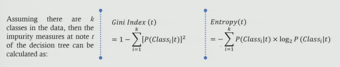
Why Impurity? Impurity = randomness in a node. A pure node = all observations belong to one class → perfect prediction. The lower the impurity at each leaf node, the higher the accuracy of classification. Goal at every split: choose the variable + cutoff that reduces impurity the most.

Formulas

• Gini Index Formula: Gini(t) = 1 − Σᵢ [ P(class i | node t) ]²
  • For binary (k=2): Gini(t) = 1 − (p₁² + p₂²)
  • Range: 0 (perfectly pure) to 0.5 (50-50 split - maximum impurity)
• Entropy Formula: Entropy(t) = − Σᵢ P(class i | node t) × log₂[ P(class i | node t) ]
  • Range: 0 (perfectly pure) to 1 (50-50 split - maximum impurity)

Gini and Entropy values for key scenarios

Scenario	Class 1 (%)	Class 2 (%)	Gini Index 1 − Σp²	Entropy -Σp·log₂(p)	Impurity Level
All in Class 1	100%	0%	1 − (1² + 0²) = 0	−(1·log₂1 + 0·log₂0) = 0	Zero ✓ (Pure)
All in Class 2	0%	100%	1 − (0² + 1²) = 0	−(0·log₂0 + 1·log₂1) = 0	Zero ✓ (Pure)
50-50 Split	50%	50%	1 − (0.5² + 0.5²) = 0.5	−(0.5·log₂0.5 + 0.5·log₂0.5) = 1	Maximum ✗
Node 0 (Root)	64%	36%	1 − (0.64² + 0.36²) = 0.46	-	High (near max)

Key Insight from Impurity Graph

Both impurity measures form an inverted U - zero when a node is pure (p = 0 or 1) and maximal at the 50-50 split (p = 0.5). Splitting aims to move nodes away from 0.5 toward the ends.

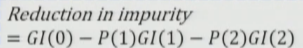
• Shape: Inverted U - symmetric around 0.5
• Both Gini and Entropy start at 0 (all in one class) → rise to maximum at 0.5 (50-50 split) → fall back to 0 (all in other class)
• Implication: When splitting a node, we want to move observations AWAY from 0.5 towards either end (0 or 1) → reduce impurity → improve accuracy

Tip

★ Exam tip: Know both formulas. Know that Gini max = 0.5 and Entropy max = 1 (for binary classification). Know that impurity = 0 means pure node. These numbers are commonly tested.

---

Splitting Logic - How to Choose Variable and Cutoff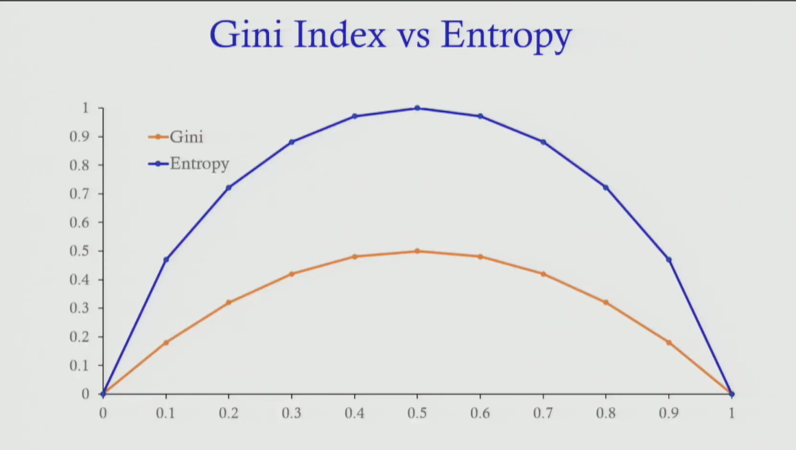

Parent nodeGini(parent)

↓  try every (variable, cutoff)

Left childw_L · Gini(left)

Right childw_R · Gini(right)

ΔImpurity = Gini(parent) − [ wL × Gini(left) + wR × Gini(right) ]

At each node the algorithm tries every variable and cutoff, then keeps the split with the largest weighted reduction in impurity (ΔImpurity).

At each node, try ALL variables (age, utilisation, MTBF, oil, etc.) with ALL possible cutoff values. For each (variable, cutoff) pair, calculate weighted reduction in impurity.

• Reduction in Impurity Formula: ΔImpurity = Gini(parent node) − [ w_left × Gini(left child) + w_right × Gini(right child) ] where w_left = (obs in left child) / (obs in parent) and w_right = (obs in right child) / (obs in parent)
• Choose: The (variable, cutoff) pair that gives the LARGEST ΔImpurity → this is the best split

Tip

★ Exam tip: Be able to compute ΔImpurity. Higher ΔImpurity = better split.

---

Node-by-Node Splitting Trace - Full Tree

Node 0 · root700 obs · Fail 447 (64%) / OK 253 (36%) · Gini 0.46

↓  best split: Oil Contamination @ 5.5

Node 1 · Oil ≤ 5.5141 obs · 33% / 67% · Gini 0.44

Node 2 · Oil > 5.5559 obs · 72% / 28% · Gini 0.40

Step 1-2: start with all training data in the root, then split on the predictor (Oil Contamination) that gives the maximum reduction in impurity.

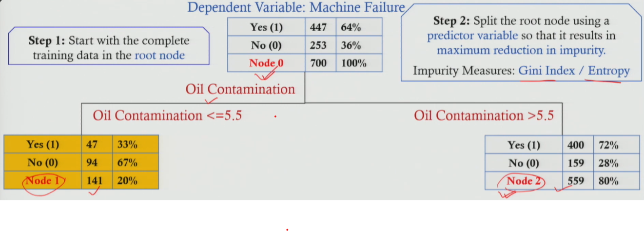
All nodes - observations, Gini, splitting variable, cutoff, impurity reduction

Node	Obs. Count	Yes% / No%	Gini	Split Variable	Cut-off	Reduction in Impurity	Child Nodes
0 (Root)	700 total (447 Yes, 253 No)	64% / 36%	0.46	Oil Contamination	5.5	0.052 (Maximum)	→ Node 1, Node 2
1	141 total	Oil ≤ 5.5	0.44	Utilisation	92.05%	0.38 (Max at Node 1)	→ Node 3, Node 4
2	559 total (72% Yes)	Oil > 5.5	0.40	MTBF	23.95	0.11 (Max at Node 2)	→ Node 5, Node 6
3 (Leaf)	109 obs.	17% / 83%	0.28	STOP	-	-	Predict: NOT FAIL
4 (Leaf)	~35 obs.	88% / 12%	0.21	STOP	-	-	Predict: FAIL
5 (Leaf)	493 obs.	77% / 23%	0.35	STOP	-	-	Predict: FAIL
6 (Leaf)	66 obs.	29% / 71%	0.41	STOP	-	-	Predict: NOT FAIL

Accuracy Progression - How Each Split Improves Prediction

Node 0 · no info64% baseline

→

+ Oil > 5.572% (+8)

→

+ MTBF ≤ 23.9577% (+5)

→

Node 4 · best leaf88% - Oil ≤ 5.5 & Util > 92.05

Each split adds information and lifts accuracy above the 64% baseline - but each additional split adds less than the last (diminishing returns), which is why the tree eventually stops.

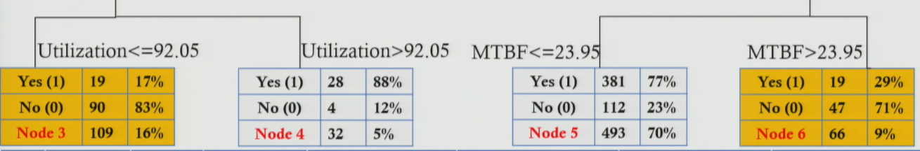
Stage	Information Available	Best Prediction Accuracy	Interpretation
Node 0 (No info)	None - just know the machine exists	64% (baseline)	64% chance it will fail based solely on history.
After Split 1 (Node 2)	Oil Contamination > 5.5	72% (+8%)	Knowing oil is high contamination improves accuracy.
After Split 2 (Node 5)	Oil > 5.5 AND MTBF ≤ 23.95	77% (+5%)	Adding MTBF info pushes accuracy further to 77%.
Node 4 (Best leaf)	Oil ≤ 5.5 AND Utilisation > 92.05%	88% (+24%)	Highest accuracy leaf - overutilised machines very likely to fail.

Key takeaway: Each split adds information → accuracy increases. Each additional split adds less accuracy improvement than the previous one (diminishing returns) → reason to stop.

---

Stopping Criteria & Overfitting

Why Stopping is Critical - Overfitting: If no stopping: Tree keeps splitting → eventually each leaf has just 1 observation → 100% accuracy on training data.

• Problem: Model “memorised” training data instead of learning patterns → poor accuracy on new test data (Overfitting).
• Fix: Apply stopping criteria to produce a simpler, more general model.

Three stopping criteria used in classification trees

Stopping Criterion	Definition	How Used in This Example
Max Tree Depth	Stop splitting once the tree reaches a pre-set maximum depth.	Depth = 2 used. No further splitting beyond that.
Min. Observations per Node	Do not split a node if it contains fewer than a minimum number (or %) of training observations.	Node 6 has ~9% and Node 4 has ~5%, triggering stop if min=10%.
Min. Reduction in Impurity	Do not split if the gain in purity is below a set threshold (epsilon).	Prevents tiny, meaningless splits.

Note

★ Stopping criteria prevent overfitting. A good model accurately predicts UNSEEN data, not perfectly fitting training data.

---

4-Step Algorithm - How to Build a Classification Tree

1. Start at root: Place all training data in the root node (Node 0). Calculate initial Gini (or entropy).
2. Find best split: For each node, try all possible (variable, cutoff) combinations. Select the one that gives maximum reduction in impurity (ΔImpurity).
3. Repeat: Apply Step 2 to each new internal node created. Keep splitting until a stopping criterion is met.
4. Stop and classify: At each leaf node, assign the majority class as the prediction. Report probability = proportion of that class in the leaf, and support = proportion of training data in that leaf.

---

Session Summary

• Root node baseline: 700 obs | 64% failure rate | Gini = 0.46 - high impurity, needs improvement
• Impurity measures: Gini Index = 1 − Σp² | Entropy = −Σp·log₂(p). Both = 0 for pure nodes, maximum at 50-50 split.
• Splitting criterion: Choose (variable, cutoff) with maximum ΔImpurity
• Accuracy progression: 64% (baseline) → 72% (after oil split) → 77%/88% (after 2nd split)
• Stopping criteria: Max depth | Min observations per node | Min ΔImpurity
• Overfitting: No stopping → 100% training accuracy but poor test accuracy. Stopping = essential for generalisation.
• Next session: Python hands-on - implement this exact model in code, reproduce the same output