Week 11 | Session 4: SC Digital Twin — Network Optimization (Excel + AnyLogistix)

Course: Supply Chain Digitization — Module 4: Digital Infrastructure

---

Session Agenda

Note

• Context — Moving from GFA to Network Optimization
• GFA vs Network Optimization — Comparison
• Case Study — Pharma Company Network Redesign
• Decision Variables
• Objective Function — Maximize Profit
• Constraints
• Excel Solver — Setup & Results
• Optimal Solution — Results
• AnyLogistix — Network Optimization Module

---

1. Context — Moving from GFA to Network Optimization

GFA (Sessions 2 & 3) found the optimal DC location from scratch — 1 DC, minimize transport cost.

This session: demand has doubled, a new factory is needed, and the existing DC lease is expiring. Must simultaneously decide: which factory to open, which DC to open, and how to route flows.

Note

★ Network Optimization = decide which nodes to open (binary) AND how much to flow between them (continuous). Much richer decision than GFA.

GFA vs Network Optimization — Comparison

Attribute	GFA (Sessions 2 & 3)	Network Optimization (This Session)
Question answered	WHERE to place a new DC from scratch?	Which factories/DCs to open AND how to route flows?
Objective	Minimize transportation cost	Maximize profit (Revenue − all costs)
Decision variables	xDC (lat), yDC (long) — 2 variables only	yᵢ (factory open), zⱼ (DC open), xᵢⱼ (flows), qⱼₖ (flows)
Facility options	Infinite possible coordinates	Fixed candidate locations — choose which to open
Variable type	Continuous — lat/long are real numbers	Mixed Integer — binary (yᵢ, zⱼ) + continuous (xᵢⱼ, qⱼₖ)
Solver method	GRG Non-linear (spherical distance is non-linear)	Simplex LP (all linear constraints and objective)
Cost components	Distance × demand × transport cost only	Fixed + production + inbound/outbound + transport costs

---

2. Case Study — Pharma Company Network Redesign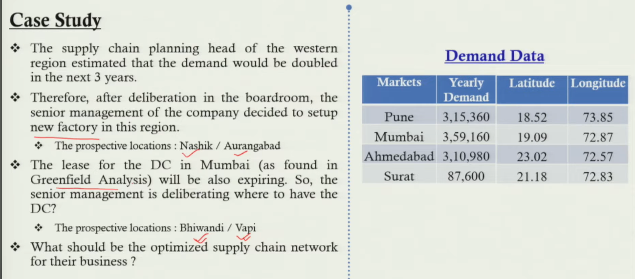

Background:

• Demand in western region will double in next 3 years — current capacity insufficient.
• Management decides to set up a new factory at one of: Nashik OR Aurangabad.
• DC in Mumbai (from GFA) lease is expiring — must relocate to one of: VAPI OR V1D (Viwandi).
• Markets remain: Pune, Mumbai, Ahmedabad, Surat — but demand is now doubled.

All Node Data

Node	Location	Prod/Proc Cost/unit	Key Distances
Factory 1	Nashik	$7/unit production	→ VAPI 144 km, → V1D 129 km
Factory 2	Aurangabad	$5/unit production	→ VAPI 322 km, → V1D 297 km
DC 1	VAPI	$0.25 inbound/outbound	→ Mumbai 169 km, Pune 298 km, Surat 102 km, Ahm 346 km
DC 2	V1D (Viwandi)	$0.50 inbound/outbound	→ Mumbai 35 km, Pune 151 km, Surat 254 km, Ahm 487 km

Transport cost: $0.001/km/unit. Revenue: $15 per unit sold.

Four Decisions to be Made Simultaneously

1. Open factory at Nashik, Aurangabad, or both?
2. Open DC at VAPI, V1D, or both?
3. Which factory supplies which DC (xᵢⱼ)?
4. Which DC serves which market — and how much (qⱼₖ)?

Note

★ All 4 decisions must be optimized simultaneously to maximize overall profit. Solving them separately gives a sub-optimal result.

---

3. Decision Variables

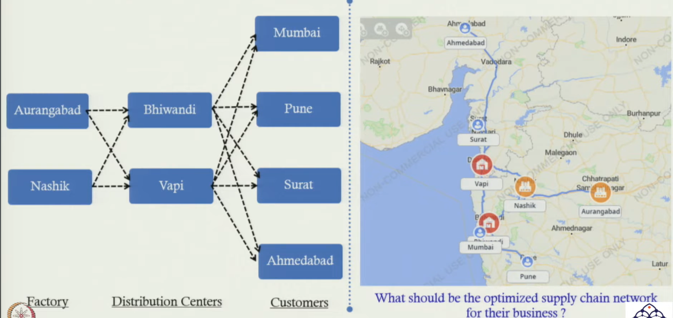
Variable	Type	Meaning
yᵢ	Binary 1	= 1 if ith factory is OPEN; = 0 if NOT open. i = 1 (Nashik), i = 2 (Aurangabad)
zⱼ	Binary 1	= 1 if jth DC is OPEN; = 0 if NOT open. j = 1 (VAPI), j = 2 (V1D)
xᵢⱼ	Continuous ≥ 0	Quantity shipped from ith factory to jth DC
qⱼₖ	Continuous ≥ 0	Quantity shipped from jth DC to kth customer (k = 1..4 markets)

Big M: a very large number. If a facility is open (y=1 or z=1), capacity = M (unlimited). If closed (=0), capacity = 0 — cannot send or receive anything.

---

4. Objective Function — Maximize Profit

Maximize Z = Revenue − Factory Fixed Cost − DC Fixed Cost
           − Production Cost − Inbound Cost − Outbound Cost
           − Factory→DC Transport Cost − DC→Customer Transport Cost

Cost / Revenue Component	Expression	Explanation
Revenue	Σⱼ Σₖ (Rev × qⱼₖ)	Rev = $15/unit. Total revenue = units sold × price.
Factory Fixed Cost	Σᵢ (FC_factory_i × yᵢ)	If yᵢ = 0: cost = 0 (factory not open). If yᵢ = 1: incur fixed cost.
DC Fixed Cost	Σⱼ (FC_dc_j × zⱼ)	If zⱼ = 0: cost = 0 (DC not open). If zⱼ = 1: incur fixed cost.
Production Cost	Σᵢ Σⱼ (PC_i × xᵢⱼ)	PC_i = production cost per unit at factory i ($7 Nashik, $5 Aurangabad).
Inbound Processing	Σᵢ Σⱼ (IB_j × xᵢⱼ)	IB_j = cost per unit for inbound processing at DC j ($0.25 VAPI, $0.50 V1D).
Outbound Processing	Σⱼ Σₖ (OB_j × qⱼₖ)	OB_j = cost per unit for outbound processing at DC j.
Factory → DC Transport	Σᵢ Σⱼ (TC × dist_ij × xᵢⱼ)	TC = $0.001/km/unit. dist_ij = km from factory i to DC j.
DC → Customer Transport	Σⱼ Σₖ (TC × dist_jk × qⱼₖ)	dist_jk = km from DC j to customer k.

---

5. Constraints

Constraint	Expression	What it Enforces
Demand satisfaction	Σⱼ qⱼₖ = Dₖ ∀k	Total shipments from all DCs to customer k must equal customer k’s full demand.
Factory capacity	Σⱼ xᵢⱼ ≤ M × yᵢ ∀i	If factory i open (yᵢ=1): can ship up to M units. If closed (yᵢ=0): capacity = 0.
DC capacity	Σₖ qⱼₖ ≤ M × zⱼ ∀j	If DC j open (zⱼ=1): can process up to M units. If closed (zⱼ=0): cannot process.
Flow balance at DC	Σᵢ xᵢⱼ = Σₖ qⱼₖ ∀j	What flows INTO each DC must equal what flows OUT. No inventory held at DC.
Binary variables	yᵢ, zⱼ ∈ 1	Factory open/close and DC open/close are binary decisions.
Non-negativity	xᵢⱼ, qⱼₖ ≥ 0	Flow quantities cannot be negative.

Note

★ Flow balance: Σᵢ xᵢⱼ = Σₖ qⱼₖ for each DC j. Total inflow = total outflow. DCs are pass-through nodes, not storage points.

---

6. Excel Solver — Setup & Results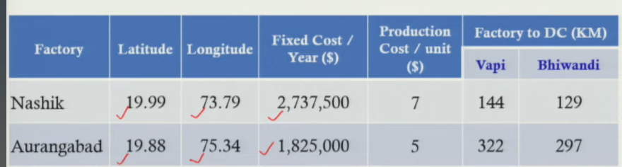

Solver Setting	Value / Detail
Set Objective	Total Profit cell (Revenue − Cost)
To	Max (Maximize)
Changing Variables	yᵢ (factory binary), zⱼ (DC binary), xᵢⱼ (factory→DC flows), qⱼₖ (DC→customer flows)
Constraint 1	DC inflow ≤ DC capacity (= M×zⱼ)
Constraint 2	Demand satisfaction at all 4 markets
Constraint 3	Factory outflow ≤ factory capacity (= M×yᵢ)
Constraint 4	Flow balance: DC inflow = DC outflow
Binary constraint	yᵢ and zⱼ set as binary (0 or 1 only)
Method	Simplex LP — objective and all constraints are linear
Result	Aurangabad factory: OPEN. VAPI DC: OPEN. Nashik + V1D: CLOSED. Profit = ₹59,27,495

Why Simplex LP (not GRG Non-linear)?

Distances are given as fixed inputs (km values) — not calculated via spherical formula. Objective function and all constraints are linear in the decision variables. Binary variables are handled as integer constraints — Simplex LP handles this as Mixed Integer LP.

---

7. Optimal Solution — Results

Facilities to Open:

• Factory: Aurangabad — OPEN (lower production cost $5/unit vs Nashik $7/unit)
• DC: VAPI — OPEN (lower inbound/outbound cost $0.25 vs V1D $0.50)
• Nashik factory: CLOSED. V1D (Viwandi) DC: CLOSED.

Product Flow:

• Aurangabad factory → VAPI DC → all 4 markets
• VAPI DC → Mumbai: 3,59,160 units
• VAPI DC → Pune: 3,15,360 units
• VAPI DC → Surat & Ahmedabad: demand matched exactly.

Optimal Profit: ₹59,27,495 — identical from Excel Solver and AnyLogistix.

Note

★ Aurangabad + VAPI selected because: lower production cost at Aurangabad + lower DC processing cost at VAPI + proximity to high-demand markets (Mumbai, Pune, Surat).

---

8. AnyLogistix — Network Optimization Module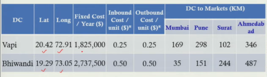

When 4 SKUs are added + daily demand → number of decision variables multiplies. Excel cannot handle large Mixed Integer Programs (MIP) efficiently. AnyLogistix has built-in MIP solver + map visualization + route details + flow breakdown.

Data Entry in AnyLogistix — Network Optimization Module

• Customers: Pune, Mumbai, Ahmedabad, Surat — 4 markets.
• Facilities: Aurangabad (factory), Nashik (factory), VAPI (DC), V1D (DC).
• Demand: per day per SKU (4 SKUs × 4 markets = 16 demand entries).
• Revenue: $15 per unit. Facility expenses: fixed cost per day.
• Objective: Revenue − Fixed cost − Inbound − Outbound − Production − Transport.
• Run → solution in seconds — same result as Excel: Aurangabad + VAPI, profit = ₹59,27,495.

Additional Outputs from AnyLogistix

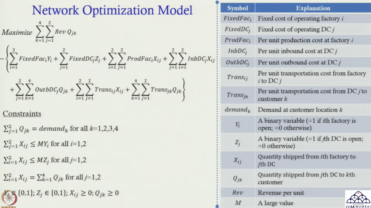
• Map visualization: actual road routes from Aurangabad → VAPI → customers.
• Flow details: Aurangabad → VAPI: SKU1 = 3,13,900 units, distance shown, transport cost shown.
• Per-route breakdown: every factory→DC and DC→customer flow with units, km, cost.
• Multiple cost layers: processing cost, flow cost, transport cost shown separately per arc.

Note

★ AnyLogistix shows the actual road route — not just straight-line connections. Key for real-world delivery planning where road distance > straight-line distance.

---

Session Summary

• Context: demand doubled → need new factory + DC. Candidates: Nashik/Aurangabad (factory), VAPI/V1D (DC).
• 4 decisions: which factories to open (yᵢ), which DCs to open (zⱼ), factory→DC flows (xᵢⱼ), DC→customer flows (qⱼₖ).
• Objective: Maximize Profit = Revenue − all 7 cost components (fixed + variable + transport).
• Big M trick: if facility closed (0) → capacity = 0 → cannot send/receive. Open (1) → capacity = M (unlimited).
• Flow balance: inflow to DC = outflow from DC. DCs are pass-through — no inventory held.
• Solver: Simplex LP (linear model, binary integer constraints). Contrast with GFA which used GRG Non-linear.
• Result: Aurangabad factory + VAPI DC. Profit = ₹59,27,495. Identical from Excel and AnyLogistix.

Tip

★ Exam Tip: 4 decision variables in network optimization: yᵢ (factory open/close, binary), zⱼ (DC open/close, binary), xᵢⱼ (factory→DC flow, continuous), qⱼₖ (DC→customer flow, continuous).

★ Exam Tip: Big M constraint: Σⱼ xᵢⱼ ≤ M × yᵢ. If yᵢ=0 → capacity=0 → cannot ship. If yᵢ=1 → capacity=M (unlimited). Replace M with actual capacity to add real capacity limits.

★ Exam Tip: Flow balance at DC: Σᵢ xᵢⱼ = Σₖ qⱼₖ for each j. All inflow must equal all outflow — DCs don’t hold inventory. This is unique to multi-tier network models.

★ Exam Tip: Network optimization solver = Simplex LP (linear). GFA solver = GRG Non-linear (spherical distance formula). Knowing WHY each method is used is key.