Week 7 | Session 5: Model Evaluation, Overfitting, Random Forest & Error Metrics

Course: Supply Chain Digitization — Module 3: Analytics in SCM

---

Session Agenda

Note

• Model performance measurement — MSE on test data (300 obs)
• Can we reduce MSE? — effect of increasing tree depth
• Overfitting — training vs. test MSE simulation across depths 2–12
• Optimal tree depth = 5
• Random Forest — concept, bootstrap sampling, feature randomisation
• Random Forest vs. single regression tree — MSE comparison
• Error metrics — MSE, MAD, MAPE, Bias, Tracking Signal
• Model selection framework — 7-step process

---

Step 1 — Measuring Model Performance on Test Data

Test data: 300 observations held out from the 1000-retailer dataset. NEVER used during training. For each of the 300 retailers: yᵢ = actual order quantity | ŷᵢ = predicted by regression tree

• MSE formula (test data): MSE = (1/n) × Σᵢ₌₁ⁿ (yᵢ − ŷᵢ)²
• Result at depth = 2: MSE (test) = 56,62,511
• Result at depth = 2 (training): MSE (train) = 59,96,464

Note

★ ALWAYS evaluate model on TEST data — not training data. Training MSE will always decrease as the model grows more complex. Test MSE shows how the model performs on NEW, unseen retailers.

Python Code for Test Prediction and MSE

from sklearn.metrics import mean_squared_error

# Predict on test data
y_pred_test = reg_tree.predict(X_test)

# Compute MSE on test data
mse_test = mean_squared_error(Y_test, y_pred_test)
print("Test MSE:", mse_test)
# Output: Test MSE: 5662511.xx

---

Overfitting — Training vs. Test MSE Simulation

Hypothesis: If we split nodes more (deeper tree) → more refined segments → lower MSE.

• For TRAINING data: Yes — MSE always decreases as depth increases.
• For TEST data: Initially decreases → then increases. Model starts memorising the training retailers instead of learning general patterns → fails on new retailers. This is Overfitting.

MSE values at each depth

Tree Depth	Training MSE	Test MSE	Interpretation
2 (baseline)	59,96,464	56,62,511	Starting point. Test MSE slightly lower than training.
3, 4	↓ Reduced	↓ Reduced	Both improving — more splits helping.
5 ← Optimal	↓ Reduced	Minimum ★	Best test performance. Optimal tree depth = 5.
6	↓ Still reducing	↑ Starts rising	OVERFITTING BEGINS. Test performance degrades.
7–12	↓ → 0 (memorising)	↑ Keeps rising	Severe overfitting. Test prediction useless.

Tip

★ Exam tip: Overfitting is always asked. Define it → show the training vs. test MSE pattern → state that the solution is to use stopping criteria (max depth, min obs) OR switch to an ensemble method like Random Forest.

---

Random Forest Algorithm — The Solution to Overfitting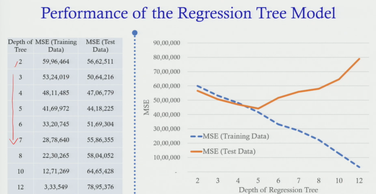

Random Forest = many decision trees built on randomised subsets of data and features. Ensemble modelling: Instead of 1 model → build k models → combine predictions. Averaging across many trees cancels out individual errors → more accurate and stable.

Two Sources of Randomness

1. Bootstrap Sampling: Draw k random samples WITH REPLACEMENT. Each tree trains on a different sample (some retailers repeated, some left out).
2. Feature Randomisation: Each tree uses a random subset of features (e.g. 3 out of 10). Different trees focus on different aspects.

4-step algorithm

1. Bootstrap sampling: Create k different training samples.
2. Randomise features: Each tree uses a random subset of features.
3. Build k trees: Build k regression trees → each gives one predicted demand (ŷ).
4. Combine predictions: Average of k predicted demands: Ŷ_final = (ŷ₁ + ŷ₂ + … + ŷₖ) / k

Note

★ Random Forest vs. Single Decision Tree: Single tree = easy to interpret but prone to overfitting. Random Forest = harder to interpret (20+ trees) but much more accurate and robust on new data.

Results — Random Forest vs. Single Regression Tree

Model	Max Depth	Test MSE	Better?
Single Regression Tree (depth 2)	2	56,62,511	Reference
Single Regression Tree (depth 5)	5	~44,xx,xxx	Better than depth 2
Random Forest (20 trees, depth 5)	5 (per tree)	37,21,603 ★	Best ✓ (~34% lower than depth 2)

---

Demand Forecast Error Metrics — All 5 Measures

Error term: eₜ = Fₜ − Dₜ (where Fₜ = Forecasted, Dₜ = Actual)

Metric	Full Name	Formula	When to Use / Interpretation
MSE	Mean Squared Error	(1/n) × Σ(Fₜ − Dₜ)²	Penalises large errors. Good for model comparison. Not in original units.
MAD	Mean Absolute Deviation	(1/n) × Σ|Fₜ − Dₜ|	Easier to interpret (same units as demand). More robust to outliers.
MAPE	Mean Absolute % Error	(100/n) × Σ|Fₜ − Dₜ| / Dₜ	Most interpretable for management (“off by X% on average”). Scale-independent.
Bias	Forecast Bias	(1/n) × Σ(Fₜ − Dₜ)	Measures systematic over/under-estimation. Should be close to 0.
Tracking Signal	Tracking Signal	Bias / MAD	Signals whether model is drifting. Triggers review if outside ±4 to ±6.

Tip

★ Exam tip: Know all 5 metrics with formulas and when each is preferred. MSE and MAPE are most commonly tested. Bias and Tracking Signal are about systematic error direction.

---

Model Selection Framework — 7-Step Process

#	Step	Example from This Course
1	Understand the data	7 retailer features: encoded categoricals. Checked for outliers.
2	Choose evaluation metric	MSE chosen. MAPE better for management reporting.
3	Split data	70% training | 30% test. Test data used ONLY for final evaluation.
4	Experiment with multiple algorithms	Tried regression tree vs. random forest. RF wins.
5	Hyper-parameter tuning	Tested depths 2–12 to find optimal depth=5.
6	Consider interpretability	Single tree: very interpretable. Random forest: harder to explain but more accurate.
7	Check resource constraints	20-tree random forest is manageable. 1000+ tree XGBoost may need cloud.

---

Module 3 — Complete Summary

• Analytics + Big Data: Data → Model → Decision → Value. Big Data 6 Vs.
• Types of Analytics: Descriptive → Diagnostic → Predictive → Prescriptive.
• Predictive Maintenance: Classification tree (Gini). Output: 4 leaf node rules. Python implementation.
• Demand Forecasting: Regression tree (MSE). Output: continuous order quantities. Python: Dummy variables.
• Random Forest & Evaluation: Overfitting, Bootstrap, Error metrics (MSE, MAD, MAPE).