Week 11 | Session 2: SC Digital Twin - Green Field Analysis (GFA) with Excel & AnyLogistix

Course: Supply Chain Digitization - Module 4: Digital Infrastructure

Session Agenda

1. What is Green Field Analysis (GFA)?

This session builds a small SC digital twin to perform GFA - finding the optimal DC location using:

Excel + Solver for small-scale problems (understanding the mechanics).
AnyLogistix software for large-scale, real-world problems.

2. Case Study - Pharma Company: DC Location for Western India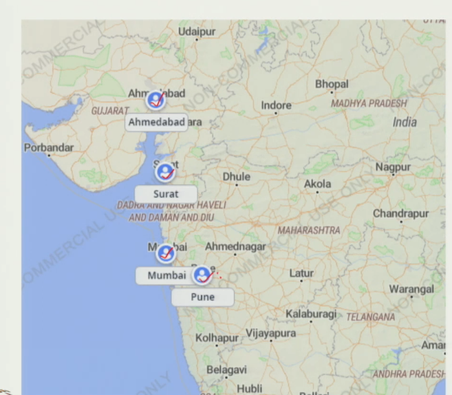

A pharmaceutical company wants to set up 1 Distribution Center to serve the western region of India.

Objective: find DC location (latitude, longitude) that minimizes total transportation cost.

Market Data

Market	Index	Annual Demand (units)	Latitude (xᵢ)	Longitude (yᵢ)
Pune	1	1,57,680	18.52	73.85
Mumbai	2	1,79,580	19.09	72.87
Ahmedabad	3	1,55,490	23.02	72.57
Surat	4	43,800	21.18	72.83

Cost assumption: $1 per km per unit of demand transported.

3. Problem Framing - Why Intuition is Insufficient

DC placed near…	Problem
Mumbai (highest demand)	Cost to Ahmedabad and Surat increases sharply
Pune	Cost to Mumbai, Ahmedabad, Surat all increase
Ahmedabad	Cost to Mumbai, Pune, Surat all increase

Conclusion: there is a trade-off - need an optimization model. Infinite possible DC locations exist; cannot evaluate manually.

4. Optimization Model - Formulation

Haversine (great-circle) distance

a = sin²(Δlat/2) + cos(lat₁)·cos(lat₂)·sin²(Δlon/2)
c = 2·atan2(√a, √(1−a))
distance = R·c  (R = earth’s radius = 6371 km)

In our context

Δlat = x_DC − xᵢ  ·  Δlon = y_DC − yᵢ
distance((xᵢ, yᵢ), (x_DC, y_DC)) = R·c

The Haversine formula gives the true over-the-earth distance between two latitude/longitude points - used to measure each market’s distance from a candidate DC location.

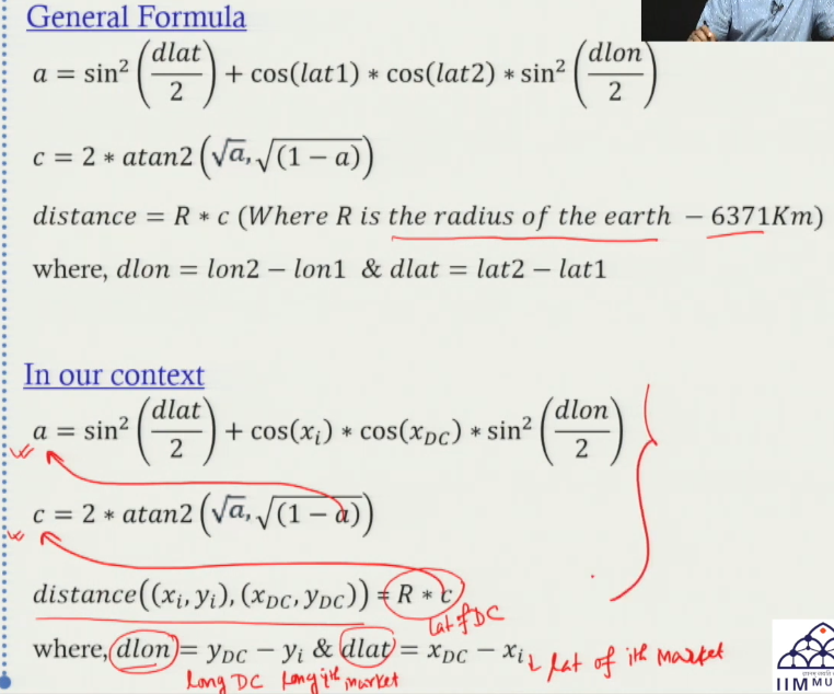
Decision Variables:

xDC = latitude of the new DC (unknown)
yDC = longitude of the new DC (unknown)

Objective: Minimize Z

Z = Σ(i=1 to 4) [ Demand_i × d(xᵢ,yᵢ → xDC,yDC) × Cost per km per unit ]

Component	Detail
Distance formula	Haversine / Spherical - accounts for earth’s curved surface → gives accurate km distance
Solver method	GRG Non-linear - because the spherical distance formula is non-linear
Constraints	None - DC can be placed at any (xDC, yDC) coordinate

5. Distance Formulas - Three Methods

Method	Formula	Accuracy
Direct Line (Euclidean)	√[(xᵢ−xDC)² + (yᵢ−yDC)²]	Low - straight-line, not realistic
Corner (Manhattan)	\|xᵢ−xDC\| + \|yᵢ−yDC\|	Medium - accounts for turns, flat grid only
Spherical (Haversine)	Haversine / Spherical trig formula	High ✓ - used in this case

Why Spherical Formula is Used

Earth’s surface is not flat - lat/long are coordinates on a curved surface. The spherical formula captures earth’s curvature → most accurate real-world km distance. It makes the objective function non-linear → must use GRG Non-linear solver (not Simplex LP).

6. Solving in Excel - Step-by-Step

Enter market data: Input demand, latitude, longitude for all 4 markets (Pune, Mumbai, Ahmedabad, Surat).
Set initial DC location: xDC = 20 (latitude), yDC = 72 (longitude) - random starting values; not the answer yet.
Calculate distances: Apply spherical distance formula from each DC location to each market → 4 distance values.
Calculate individual costs: Cost_i = Demand_i × Distance_i × $1 (cost per km per unit).
Calculate total cost Z: Z = Sum of all 4 individual costs. At initial (20, 72): Z = 12,44,89,119.
Run Solver: Set objective = minimize total cost cell. Changing variables = latitude cell, longitude cell. Method = GRG Non-linear. Solve.
Read optimal solution: Optimal xDC = 19.09, yDC = 72.87. Total cost = 9,73,92,135. Location = Mumbai.

Cost Calculation at Initial Location (20, 72)

Route	Calculation	Cost
DC → Pune	1,57,680 × 254.543 km × $1	4,01,59,298
DC → Mumbai	1,79,580 × 136.197 km × $1	2,44,58,875
DC → Ahmedabad	1,55,490 × 340.945 km × $1	5,29,98,141
DC → Surat	43,800 × 157.099 km × $1	68,80,136
Total Z		12,44,89,119

Optimal Solution from Solver

Excel setup - with a trial DC at (20.00, 72.00), the Haversine distance to each market and the total distance-weighted cost:

Market	Cost/km·unit	Demand (units)	Latitude	Longitude	Distance (km)
Pune	1	157,680	18.52	73.85	254.54
Mumbai	1	179,580	19.09	72.87	136.20
Ahmedabad	1	155,490	23.02	72.57	340.95
Surat	1	43,800	21.18	72.83	157.10
Trial DC (20.00, 72.00)					Cost = 124,489,119

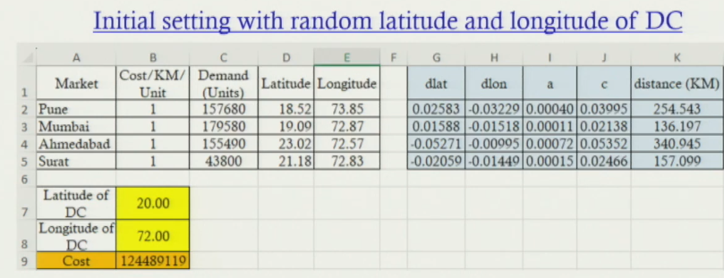
Parameter	Value
Optimal DC latitude (xDC)	19.09
Optimal DC longitude (yDC)	72.87
Optimal location	Mumbai
Minimized total cost Z	9,73,92,135
Cost saving from optimization	~₹2.7 crore / year

7. Digital Twin Visualization - What it Adds

The Excel model gives the coordinates - but no visual map of the SC. Digital twin visualization adds:

Exact geographic position of each market plotted using lat/long.
DC location plotted at the optimized coordinates.
Routes from DC to each market shown - visual confirmation of the network.
Immediate intuition about coverage area and travel paths.

This is what tools like AnyLogistix provide - map-based visualization + optimization combined.

8. Scaling Up - AnyLogistix Software for Large Problems

Why Excel Fails at Scale

Excel works for 4 markets - but 4,000 or 40,000 markets make it impractical. Manual lat/long entry for thousands of cities is not feasible. Formula setup, solver configuration, and interpretation become unmanageable.

How AnyLogistix Solves This

Attribute	Excel Solver	AnyLogistix (DT software)
Scale	Small (4 markets - manageable manually)	Large (thousands of markets - nationwide / global)
Lat/Long input	Must be manually entered for each location	Enter city name → auto-retrieves lat/long from database
Visualization	Basic - no map plotting built in	Plots all nodes on actual map automatically after input
Algorithm	Non-linear Solver (GRG) - user sets it up	Built-in optimization algorithm runs automatically
Result output	Optimal xDC, yDC + total cost (cell values)	Optimal DC location plotted on map + lat/long + connections
Speed	Feasible but manual - formula setup required	Click of a button - fully automated for any scale
Typical use	Teaching, small-scale understanding	Real-world SC network design and digital twin development

AnyLogistix result confirmed: GFA optimal DC = lat 19.09, long 72.87 = Mumbai - matches Excel Solver output exactly.

9. Digital Twin Framework Applied to This Example

Digital Visualization: 4 markets + optimal DC location plotted on geographic map with routes.
Digital Technology: AnyLogistix software + optimization algorithm (connects physical SC problem to digital model).
Prescriptive Analytics: model tells WHERE to locate DC to minimize cost - a direct prescriptive output.

This is a full mini digital twin - not just a visualization, but an analytically driven location decision.

Session Summary

GFA: finding optimal location for a NEW DC using optimization - a prescriptive analytics application.
Case: pharma company, 4 western India markets (Pune, Mumbai, Ahmedabad, Surat), minimize transportation cost.
Model: Minimize Z = Σ(Demand_i × Distance_i × Cost/km/unit). Decision variables: xDC, yDC.
3 distance formulas: Direct line (low acc) → Corner/Manhattan (medium) → Spherical/Haversine (high - used here).
Spherical formula = non-linear → must use GRG Non-linear solver (not Simplex LP).
Excel result: Optimal xDC = 19.09, yDC = 72.87 (Mumbai). Cost = ₹9.73 Cr vs ₹12.44 Cr at random start.
AnyLogistix: same result plotted on map automatically - scales to thousands of markets.
DT components used: Visualization (map) + Technology (AnyLogistix) + Prescriptive Analytics (location optimization).