Week 8 | Session 5: SC Network Design — LP Optimization & Final Comparison
Course: Supply Chain Digitization — Module 3: Analytics in SCM
Session Agenda
Section titled “Session Agenda”1. Recap — Same Problem, Better Method
Section titled “1. Recap — Same Problem, Better Method”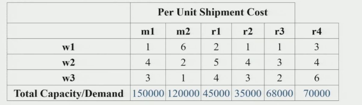
Same SC network as Session 4: 2 Manufacturers, 3 Warehouses, 4 Retailers, 1 product.
- Objectives: Find optimal distribution strategy to satisfy retailer demand and minimize total distribution costs.
- Session 4: Solved using Heuristic 1 (₹9,61,000) and Heuristic 2 (₹7,57,000).
- This session: Solve using Linear Programming (LP) + Excel Solver to get the true optimal.
2. LP Formulation — SC Network Design
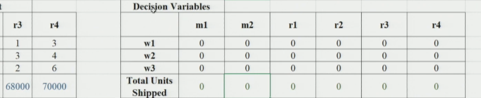
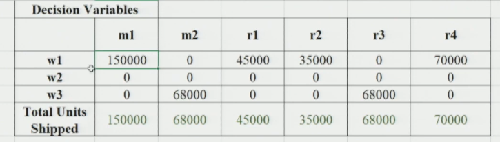
Section titled “2. LP Formulation — SC Network Design”Decision Variables — 18 total
Section titled “Decision Variables — 18 total”- 6 variables (M→W tier): Quantity moved between each Manufacturer–Warehouse pair (e.g.,
QM1W1). - 12 variables (W→R tier): Quantity moved between each Warehouse–Retailer pair (e.g.,
XW1R1).
All initialized to 0 in Excel — Solver finds the optimal values.
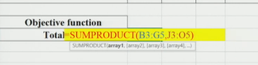
3. Objective Function
Section titled “3. Objective Function”Minimize total distribution cost = sum of (unit shipping cost × quantity) for all pairs.
(In Excel: use SUMPRODUCT)
Minimize Z = Σ (Shipping Cost × Q_MiWk) + Σ (Shipping Cost × X_WkRj)
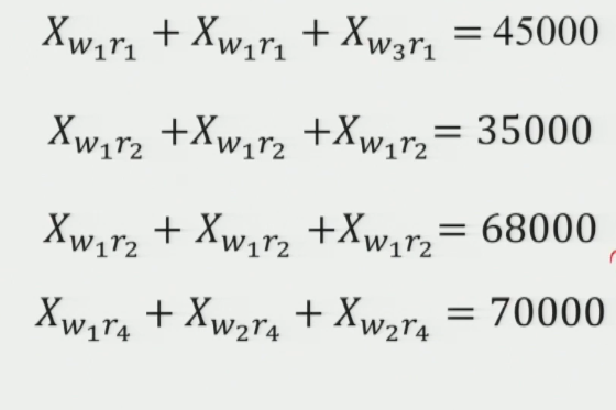
4. Constraints
Section titled “4. Constraints”Three types of constraints — all must be satisfied simultaneously for a valid solution.
| Constraint Type | Expression | What it ensures |
|---|---|---|
| Supply (2) | QM1W1+QM1W2+QM1W3 ≤ 1,50,000 | Total shipped from each Mfr ≤ its capacity |
| Flow Balance (3) | Σ(in to W1) = Σ(out of W1) | What comes into a WH must go out — no stockpiling |
| Demand (4) | XW1Rj+XW2Rj+XW3Rj = Dj | All three WHs together must fulfill each retailer’s demand |
| Non-negativity | All Q and X variables ≥ 0 | Quantities cannot be negative |
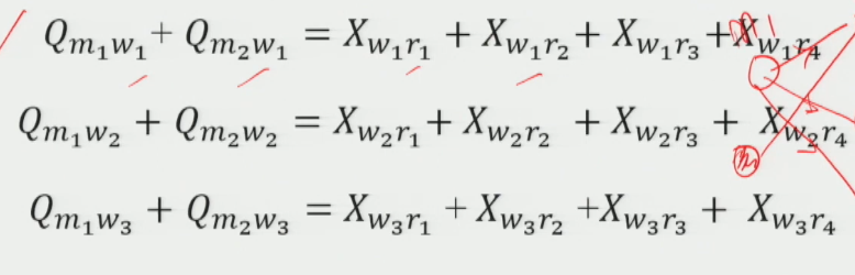
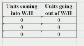
Flow Balance Constraint — Key New Concept
Section titled “Flow Balance Constraint — Key New Concept”Ensures warehouses are pass-through nodes — they do not hold inventory.
For W1: QM1W1 + QM2W1 = XW1R1 + XW1R2 + XW1R3 + XW1R4
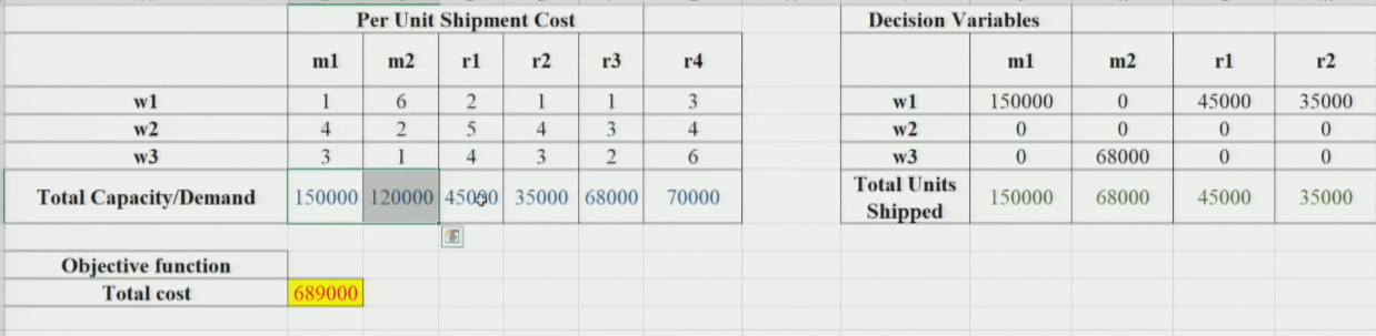
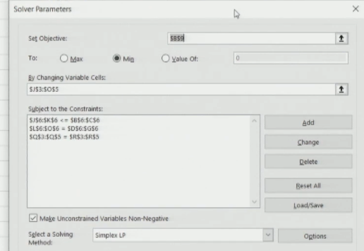
5. Solving in Excel — Step-by-Step
Section titled “5. Solving in Excel — Step-by-Step”- Set Objective: Select the Total Cost cell → choose Minimize.
- Changing Variable Cells: Select ALL decision variable cells (18 cells).
- Add Constraints: Add supply, flow balance, and demand constraints.
- Non-negativity: Check ‘Make unconstrained variables non-negative’.
- Solving Method: Select Simplex LP (model is fully linear).
- Solve: Click Solve → Keep Solver Solution.
6. Result & Final Comparison
Section titled “6. Result & Final Comparison”LP Optimal Solution
Section titled “LP Optimal Solution”Solver confirms: all constraints and optimality conditions satisfied. Total Distribution Cost = ₹6,89,000 ← global optimum.
Approach Comparison
Section titled “Approach Comparison”| Approach | Method | Total Cost | Optimal? | Savings vs H1 |
|---|---|---|---|---|
| Heuristic 1 | Cheapest WH for all | ₹9,61,000 | No | — |
| Heuristic 2 | Cheapest path per retailer | ₹7,57,000 | No | ₹2,04,000 |
| LP Optimization | Simplex LP via Excel Solver | ₹6,89,000 | Yes — guaranteed | ₹2,72,000 |
Session Summary
Section titled “Session Summary”- Problem: 2 Mfr → 3 WH → 4 Retailers, minimize total shipping cost.
- Decision Variables: 6 (Mfr→WH) + 12 (WH→Retailer) = 18 total.
- 3 Constraints: Supply (≤ capacity) | Flow Balance (in = out at WH) | Demand (= retailer req).
- Solver: Simplex LP.
- Result: LP = ₹6,89,000 (optimal). Beats heuristics significantly.