Week 8 | Session 1: SC Network Optimization — Facility Selection & Break-Even Analysis
Course: Supply Chain Digitization — Module 3: Analytics in SCM
Session Agenda
Section titled “Session Agenda”1. Module Context — Analytics in Supply Chain
Section titled “1. Module Context — Analytics in Supply Chain”- Data availability has increased → analytics now critical for SC decisions
- This week focuses on Supply Chain Network Optimization
- We explore the role of facilities in SC design and how these decisions affect customer demand fulfillment.
2. SC Network Design — Objective & Key Trade-offs
Section titled “2. SC Network Design — Objective & Key Trade-offs”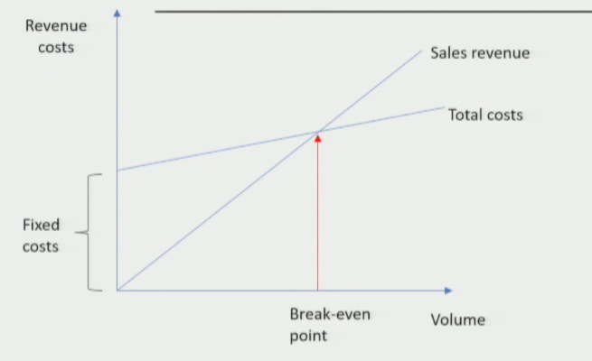
Objective: Minimize SC cost, improve service levels, fulfill customer demand optimally.
Efficient vs Responsive SC — Quick Recap
Section titled “Efficient vs Responsive SC — Quick Recap”- Efficient SC: Fewer facilities, larger in size.
- Responsive SC: More facilities, smaller in size.
Key question: How many? And where? → This is the network optimization problem.
3. Factors Affecting Facility Location
Section titled “3. Factors Affecting Facility Location”| Factor | Description |
|---|---|
| Demand | Volume, frequency, customer location — quantified from market data |
| Suppliers | Type, location, availability of suppliers for your product |
| Logistics Infrastructure | Existing roads, ports, rail — affects viability of location |
| Labour | Availability & cost of workforce at that location |
| Regulations / Tax Benefits | Government incentives change over time — must be factored in |
Facilities in SC can be: manufacturing plant, warehouse, distribution center, retailer, etc.
4. Three Major Decisions in SC Network Optimization
Section titled “4. Three Major Decisions in SC Network Optimization”- Facility Selection Decision — Choose best from existing/available options.
- Facility Location Decision — Find exact location for a new facility given supply/demand constraints.
- Complete SC Network Design — Design entire network using an optimization approach.
Today’s focus: Facility Selection using Break-Even Analysis.
5. Break-Even Analysis (BEA) — Concept
Section titled “5. Break-Even Analysis (BEA) — Concept”Definition: Identifies the level of activity at which a company is neither at profit nor at loss. The point where Sales Revenue = Total Cost is the Break-Even Point (BEP).
Two Types of Cost
Section titled “Two Types of Cost”- Fixed Cost (FC): One-time, independent of volume (Machinery, buildings, R&D).
- Variable Cost (VC): Changes with volume of production (Raw material, packaging, direct labour).
Formulas
Section titled “Formulas”Total Cost = Fixed Cost + (Variable Cost per unit × Quantity)BEP = Fixed Cost ÷ (Revenue per unit – Variable Cost per unit)
6. Case Study — Luggage Bag Company: Warehouse Location Decision
Section titled “6. Case Study — Luggage Bag Company: Warehouse Location Decision”Problem Statement:
- Company is launching a new bag category based on customer demand.
- Estimated demand = 1,45,000 units.
- Goal: identify the most cost-effective warehouse location among 3 options.
| Location | City | Fixed Cost (₹) | Variable Cost (₹/unit) |
|---|---|---|---|
| X | Noida | 1,45,000 | 11 |
| Y | Lucknow | 4,50,000 | 7 |
| Z | Chandigarh | 7,80,000 | 6 |
7. Applying Break-Even Analysis — Step-by-Step
Section titled “7. Applying Break-Even Analysis — Step-by-Step”- Enter Data: Input Fixed Cost & Variable Cost for each location in Excel.
- Assume Volume Range: Calculate Total Cost for Q = 50k to 300k.
- Calculate Total Cost:
Total Cost = FC + (VC × Q)for all 3 locations. - Plot the Graph: X-axis = Volume, Y-axis = Total Cost.
- Find Intersection Points: Identify where lines cross (break-even quantities).
- Read Decision: For 1,45,000 units, find which location line is lowest.
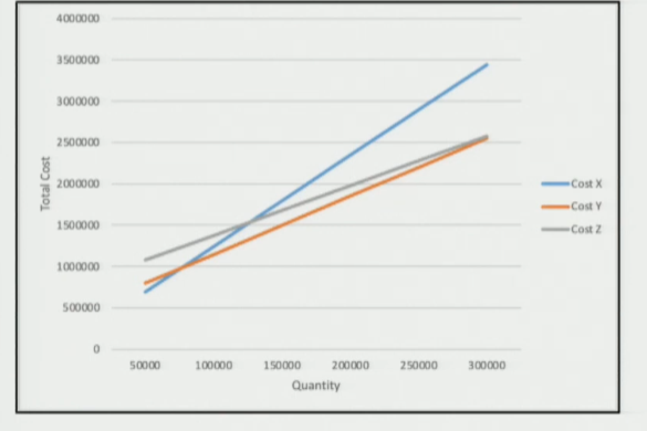
8. Result & Conclusion
Section titled “8. Result & Conclusion”- At 1,45,000 units → Location Y (Lucknow) has the lowest total cost.
- Decision: Warehouse at Lucknow (Y) is the most cost-effective choice.
Session Summary
Section titled “Session Summary”- SC Network Optimization: Strategic, long-term problem balancing cost, service level, demand fulfillment.
- Facility Location Factors: Demand, suppliers, logistics infra, labour, regulations, geography.
- Break-Even Analysis: Simple, widely-used method for facility selection from given alternatives.
- BEP Formula:
FC ÷ (Revenue/unit – VC/unit) = volume at zero profit/loss - Case Result: Location Y (Lucknow) optimal for 1,45,000 units — lowest total cost.