Week 8 | Session 2: Facility Location Decision — Centre of Gravity Method

Course: Supply Chain Digitization — Module 3: Analytics in SCM

Session Agenda

1. Recap — Facility Selection vs. Facility Location

Last session: Break-Even Analysis for facility selection — choosing best from existing options at a given volume.
This session: Facility Location Decision — finding the optimal coordinates for a brand new facility.

2. Case Study — Cooking Range Manufacturer

Background:

Manufacturer currently has a single assembly factory near Mumbai serving the entire Indian market alone.
Rapid demand growth observed → CEO decides to build a second factory.
Task for SC Manager: Find the optimal location for this new factory.

Network Structure:

Supply Sources: Parts plants in Chennai, Kolkata, Hyderabad (3 nodes)
Markets: Delhi, Bangalore, Mumbai, Pune, Chennai (5 nodes)
New Factory: (X, Y) Unknown — to be determined.

Given Data:

Coordinate locations (X, Y) of all supply sources and markets
Demand at each market and supply quantity from each parts plant
Shipping cost per unit per mile

3. Centre of Gravity Method — Concept

Centre of Gravity Method Concept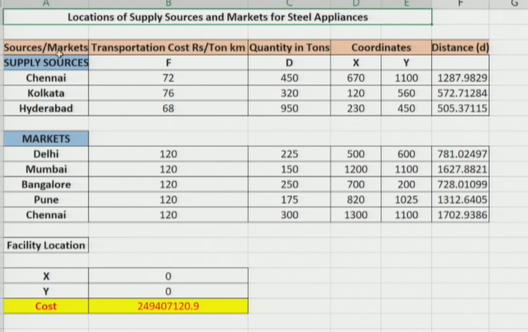

Analytical approach based on coordinate locations of supply sources & markets. Considers demand, supply quantities, and distances to find the location that minimizes total weighted transportation cost.

Variable	Meaning
X, Y	Coordinates of the new facility (decision variables — unknown)
Xi, Yi	Coordinates of supply source / market node `i`
F	Shipping cost per unit per mile
D	Quantity to be shipped
d	Distance between the new facility and a given node (calculated)

4. Key Formulas

Euclidean Distance Formula

Used to calculate the straight-line distance between the new facility (X, Y) and any node (Xi, Yi).

d = √ [ (X – Xi)² + (Y – Yi)² ]

(Applied for each of the 3 supply sources and 5 markets → 8 distances in total)

Total Transportation Cost Formula

Cost = sum of (shipping cost × quantity × distance) over ALL nodes.

Total Cost = Σ (F × D × d)

(In Excel: use SUMPRODUCT function)

5. Solving in Excel — Step-by-Step

Data Entry: Enter shipping cost (F), quantity (D), and coordinates (X, Y) for all nodes.
Define Decision Variables: Create two cells for X and Y (new factory) — initialize both to 0.
Distance Calculation: Use Euclidean distance formula for every supply source and market node.
Total Transportation Cost: Use SUMPRODUCT function: Total Cost = Σ (F × D × d)
Optimize using Solver: Data tab → Solver. Objective = minimize Total Cost. Variables = X, Y cells. Method = GRG Nonlinear.

Excel Solver Configuration

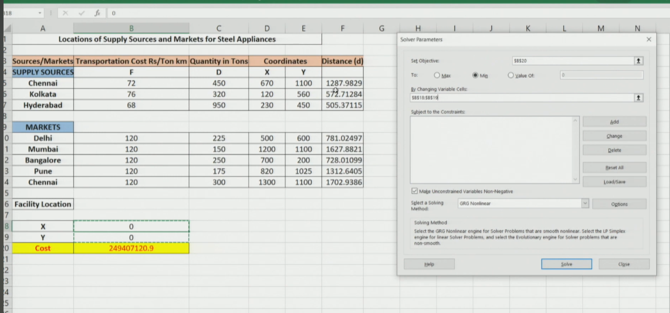
6. Excel Solver — Settings Detail

Set Objective: Select the Total Cost cell → set to Minimize.
Changing Variable Cells: Select X and Y cells (decision variables).
Solving Method: Use GRG Nonlinear — because the cost function is non-linear (due to the square root in the distance formula).

7. Result & Decision

After optimization: X ≈ 500, Y ≈ 600 (initially 0, 0)
These coordinates correspond to approximately Delhi.
Decision: Locate the new factory near Delhi to minimize total transportation cost.

What if the Optimal Location is Not Feasible?

Real-world constraints may prevent building exactly at (500, 600) due to land unavailability, regulations, lack of infrastructure, etc.
Solution: Explore nearby areas close to the optimal coordinates. Choose the nearest feasible location that meets secondary criteria (infrastructure, labour).

Session Summary

Facility Location: Strategic decision to find WHERE to build a new facility from scratch.
Centre of Gravity: Uses coordinates + demand + shipping cost to find cost-minimizing location.
Euclidean Distance: d = √[(X–Xi)² + (Y–Yi)²]
Total Cost: Σ(F × D × d) — minimized using Excel Solver (GRG Nonlinear).
Result: Optimal (X, Y) ≈ Delhi area; if infeasible, explore nearby locations.